Supp-1: Linear Algebra - 1

2021-1학기, 대학에서 ‘통계적 데이터마이닝’ 수업을 듣고 공부한 바를 정리한 글입니다. 지적은 언제나 환영입니다 :)

(Review) Matrix

✨ (중요) 별다른 언급이 없다면, 모든 벡터 “column vector“다. ✨

A $3 \times 1$ vector $\mathbf{x}$ is

\[\mathbf{x} = \begin{pmatrix} 1 \\ 2 \\ 3 \end{pmatrix}\]

<행렬; matrix>는 “vector”를 원소로 갖는 “(column) vector”다.

A $4 \times 3$ matrix $\mathbf{X}$ is

\[\mathbf{X} = \begin{pmatrix} \mathbf{x}_1^T \\ \mathbf{x}_2^T \\ \mathbf{x}_3^T \\ \mathbf{x}_4^T \end{pmatrix} = \begin{pmatrix} 1 & 2 & 3 \\ 4 & 5 & 6 \\ 7 & 8 & 9 \\ 10 & 11 & 12 \end{pmatrix}\]

• $X_i$: $X$의 $i$번째 원소 = $\mathbf{x}_i$
• $X_{ij}$: $X$의 $i$번째 원소 $\mathbf{x}_i$의 $j$번째 원소

행렬을 열벡터로 해석하는 시야👀를 체득하는게 중요하다!

Matrix Multiplication

행렬 곱셈의 시작은 좌표 변환이다.

\[\begin{pmatrix} c_1 & c_2 & c_3 & c_4 \end{pmatrix} \begin{pmatrix} x \\ y \\ z \\ t \end{pmatrix} = c_1 x + c_2 y + c_3 z + c_4 t\]

위의 예시는 간단한 거고, 조금 복잡하게 가면,

\[X \begin{pmatrix} x \\ y \\ z \\ t \end{pmatrix} = \begin{pmatrix} \mathbf{x}_1^T \\ \mathbf{x}_2^T \\ \mathbf{x}_3^T \\ \mathbf{x}_4^T \end{pmatrix} \begin{pmatrix} x \\ y \\ z \\ t \end{pmatrix} = \mathbf{x}_1^T \cdot \begin{pmatrix} x \\ y \\ z \\ t \end{pmatrix} + \mathbf{x}_2^T \cdot \begin{pmatrix} x \\ y \\ z \\ t \end{pmatrix} + \mathbf{x}_3^T \cdot \begin{pmatrix} x \\ y \\ z \\ t \end{pmatrix} + \mathbf{x}_4^T \cdot \begin{pmatrix} x \\ y \\ z \\ t \end{pmatrix}\]

좌표 변환, 또는 선형 변환의 도구로의 행렬 곱셈은

For $A \in \mathbb{R}^{n\times p}$, $\mathbf{x} \in \mathbb{R}^{p\times 1}$

\[A \mathbf{x} \in \mathbb{R}^{n\times 1}\]

즉, $p$차원 벡터를 차원 $n$으로 매핑하는 것이다. 이를 위해서는 $p$차원 벡터가 $n$개가 필요하고, 이것이 바로 행렬 $A$다…!

Definition. Design Matrix 🔥

정규 수업의 첫번째 강의에서는 <linear regression>을 수학적으로 정의하면서 <design matrix> $X$를 제시한다. 이 <design matrix>는 $p$-dim input features vector $n$개를 모은 $n \times p$ 차원의 행렬이다.

\[X = \begin{pmatrix} x_1^T \\ x_2^T \\ \vdots \\ x_n^T \end{pmatrix} \in \mathbb{R}^{n\times p}\]

<linear regression>에선 coefficients 벡터인 $\beta$를 곱해 $X \beta \in \mathbf{R}^{n\times 1}$을 구한다. 그러면 $n\times 1$의 열벡터가 나오는데, 만약 $n \ge 1,000$라면, $X\beta$가 너무 큰 차원의 벡터가 아닌가, 너어어무 큰 선형변환이 아닌가 생각했던 적이 있다. 그런데 그런 의문은 아래의 식을 보자 해결되었다.

\[Y = X\beta + \epsilon\]

즉, $X\beta$에서 $X$는 선형변환으로 사용된 것이 아니다. 오히려 <regression>을 그 자체를 수행하기 위해 고안된 “행렬”이라고 받아들이는 것이 좋다! 😁

---

Linear Algebra

Definition. Vector Space

A <vector space> is a set, consisting of vectors, equipped with scalar multiplication and vector addition.

Definition. Linear Function

For two vector spaces $V$ and $W$, a function $f: V \longrightarrow W$ is called to be <linear> if

\[f(c\mathbf{x} + \mathbf{y}) = cf(\mathbf{x}) + f(\mathbf{y}) \quad \text{for all} \; \mathbf{x}, \mathbf{y} \in V \; \text{and} \; c \in \mathbb{R}\]

Theorem.

Every <linear function between Euclidean spaces> can be represented as a matrix multiplication.

\[f(\mathbf{x}) = A \mathbf{x}\]

Note.

$n \times p$ 크기의 행렬 $A = (a_{ij})$는 <linear function from $\mathbb{R}^p$ to $\mathbb{R}^n$>으로 해석할 수 있다!!

\[f_A (\mathbf{x}) = A\mathbf{x}\]

보통 $n \times p$ 크기의 행렬에서

• $n$ = sample size
• $p$ = # of input variables

로 해석한다!

Definition. Linear Subspace

$\mathcal{L} \subset \mathbb{R}^n$ is called a <linear subspace> of $\mathbb{R}^n$ if

\[\text{For} \quad \mathbf{x}, \mathbf{y} \in \mathcal{L} \quad \text{and} \quad c \in \mathbf{R} \implies c \mathbf{x} + \mathbf{y} \in \mathcal{L}\]

Definition. span

$\mathcal{L}$ is <spanned> by ${\mathbf{x}_1, \dots, \mathbf{x}_k }$ if

\[\mathcal{L} = \left\{ c_1 \mathbf{x}_1 + \cdots + c_k \mathbf{x}_k : c_j \in \mathbb{R} \right\}\]

앞으로 이런 spanned subspace를 아래와 같이 표기한다.

\[\left[ \mathbf{x}_1, \dots, \mathbf{x}_k \right]\]

---

Definition. Linearly Independent

$\left\{\mathbf{x}_1, \dots, \mathbf{x}_k \right\}$ is called to be <linearly independent> if

\[c_1 \mathbf{x}_1 + \cdots + c_k \mathbf{x}_k = 0 \iff c_1 = \cdots = c_k = 0\]

즉, Linear Comb.가 0이 되려면, Coeffi $c_i$가 모두 0이 되어야 한다!

Theorem. T.F.A.E.

1. $\left\{\mathbf{x}_1, \dots, \mathbf{x}_k \right\}$ is linearly independent.
2. Any $\mathbf{x}_i$ cannot be represented as a linear combination of $\left\{ \mathbf{x}_j : j \ne i \right\}$.
   • 즉, \(\displaystyle \mathbf{x}_i = \sum_{j \ne i} c_j \mathbf{x}_j\)가 불가능하다는 말이다.

Definition. basis & dimension

$\left\{\mathbf{x}_1, \dots, \mathbf{x}_k \right\}$ is called a <basis> of $\mathcal{L}$ if

1. $\mathcal{L} = \left[ \mathbf{x}_1, \dots, \mathbf{x}_k \right]$
2. $\left\{\mathbf{x}_1, \dots, \mathbf{x}_k \right\}$ is linearly inependent.

Also, we call $k$ as a <dimension> of $\mathcal{L}$, $\dim(\mathcal{L})$.

Theorem.

If $\left\{\mathbf{x}_1, \dots, \mathbf{x}_k \right\}$ is a basis of $\mathcal{L}$ and $\mathbf{x} \in \mathcal{L}$, there exist unique $c_1, \dots, c_k \in \mathbb{R}$ s.t.

\[\mathbf{y} = c_1 \mathbf{x}_1 + \cdots + c_k \mathbf{x}_k\]

즉, <basis>에 의한 representation은 uniqueness를 보장한다!

Definition orthogonal & orthonormal

A basis $\left\{\mathbf{x}_1, \dots, \mathbf{x}_k \right\}$ of $\mathcal{L}$ is called to be <orthogonal> if $\mathbf{x}_i^T \mathbf{x}_j = 0$ for $i \ne j$.

If the norm of each basis $\mathbf{x}_i$ is one, then we call them as <orthonormal>.

Theorem.

If $\left\{\mathbf{x}_1, \dots, \mathbf{x}_k \right\}$ is an orthonormal basis of $\mathcal{L}$ and $\mathbf{y} \in \mathcal{L}$, then

\[\mathbf{y} = \left( \mathbf{x}_1^T \mathbf{y} \right) \mathbf{x}_1 + \cdots + \left( \mathbf{x}_k^T \mathbf{y} \right) \mathbf{x}_k\]

즉, 만약 <orthonormal basis>라면, vector $\mathbf{y}$ 를 표현하는 모든 coefficient $c_i$를 uniquely하게 특정할 수 있다는 말이다!

---

Rank Theory

Definition. Column space & Row space & Null space

\[A \in \mathbb{R}^{n \times p}\] \[A\mathbf{x} = \begin{bmatrix} \mid & \cdots & \mid \\ \mathbf{a}_1 & \cdots & \mathbf{a}_p \\ \mid & \cdots & \mid \end{bmatrix} \begin{bmatrix} x_1 \\ \vdots \\ x_p \end{bmatrix} = x_1 \mathbf{a}_1 + \cdots x_p \mathbf{a}_p\]

1. <Column space> $\mathcal{C}(A)$는 $A$의 Column으로 span한 linear space다.

= $\left[ \mathbf{a}_1, \dots, \mathbf{a}_p \right]$

= $\left\{ A\mathbf{x} : \mathbf{x} \in \mathbb{R}^p \right\}$

2. <Row space> $\mathcal{R}(A)$는 $A$의 Row로 span한 linear space다.

NOTE: $\mathcal{R}(A) = \mathcal{C}(A^T)$

3. <Null space> $\mathcal{N}(A)$는 $A\mathbf{x} = \mathbf{0}$인 모든 $\mathbf{x}$로 span한 linear space다.

= $\left\{ \mathbf{x} \in \mathbb{R}^p: A \mathbf{x} = \mathbf{0} \right\}$

NOTE: 만약 $A$가 invertible이라면, $A\mathbf{x} = \mathbf{0}$을 만족하는 $\mathbf{x}$는 $\mathbf{0}$ 뿐이기 때문에, $\mathcal{N}(A) = \mathbf{0}$이 된다.

Definition. Rank

The <rank> of $A$ is the dimension of $\mathcal{C}(A)$.

Theorem. Fundamental Theorem of Liniear Algebra

Part 1: (Rank-Nullity Theorem; Rank Theorem)

The column and row spaces of an $m \times n$ matrix $A$ both have dimension $r$, the <rank> of the matrix.

• the nullspace has dimension $n-r$
• the left nullspace has dimension $m-r$

Part 2:

The <Null space> and <Row space> are <orthogonal>.

The <Left Mull space> and the <Column space> are also <orthogonal>.

Part 3:

Any matrix $M$ can be written in the form

\[U \Sigma V^T\]

where

• $U$ is an $m\times m$ unitary matrix.
• $\Sigma$ is an $m\times n$ matrix with non-negative values on the diagonal.
• $V$ is an $n\times n$ unitary matrix.

Theorem. Rank Theorem

For any $A \in \mathbb{R}^{n \times p}$,

\[\dim (\mathcal{C}(A)) = \dim (\mathcal{R}(A))\]

그래서 <Rank Theorem>에 의해 행렬 $A$의 <rank>를 $\dim (\mathcal{C}(A))$로 정의하든, $\dim (\mathcal{R}(A))$로 정의하든 상관이 없다!

증명은 이곳을 참조할 것 👉 proof

Properties. Rank

\[A, B \in \mathbb{R}^{n\times p}\]

1. $\text{rank}(A) \le \text{rank}(n, p)$

2. $\text{rank}(A) = \text{rank}(A^T)$ (by <Rank Theorem>)

3. $\text{rank}(A) + \dim(\mathcal{N}(A)) = p$

4. If $A \in \mathbb{R}^{n\times n}$, T.F.A.E.

• $A$ is invertible
• $\text{rank}(A) = n$
• $\mathcal{N}(A) = 0$
• $\det (A) \ne 0$

5. $\text{rank}(AB) = \text{rank}(A)$ if $B$ is invertible

6. $\text{rank}(AB) = \text{rank}(B)$ if $A$ is invertible

7. $\text{rank}(AB) \le \min \{ \text{rank}(A), \text{rank}(B)\}$

8. $\text{rank}(AA^T) = \text{rank}(A^TA) = \text{rank}(A)$

---

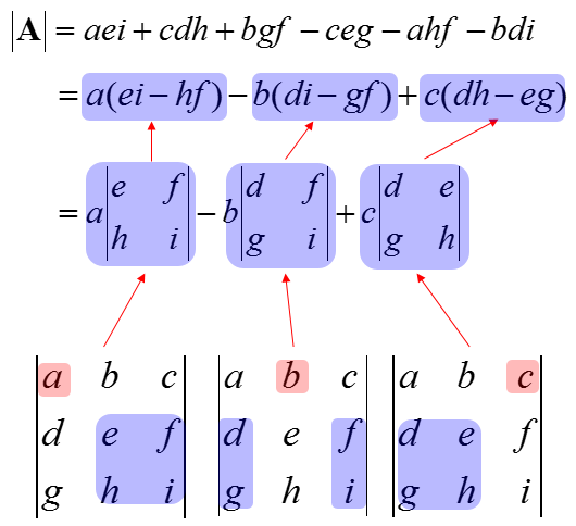
Definition. Determinant

The <determinant> of a matrix $A \in \mathbb{R}^{n \times n}$ is

\[\sum_{\pi} \text{sgn} (\pi) \cdot \left( a_{1\pi(1)} \cdots a_{n\pi(n)}\right)\]

where the summation is taken over all permutations of $\{ 1, \dots, n\}$.

<Determinant>에 대한 정말 Abstract 한 정의다. $3\times3$ 에 대해선 아래와 같이 쉽게 구할 수 있다.

Properties. Determinant

이어지는 성질들은 <Determinant>에 대한 성질을 정말 Abstract 한 용어로 기술한 것이다.

\[A, B \in \mathbb{R}^{n\times n}\]

• Multilinear (= linear for each column & row)

\[\det (\mathbf{a}_1, \dots, c\mathbf{a}_i + \mathbf{d}, \dots, \mathbf{a}_n) = c \det (\mathbf{a}_1, \dots, \mathbf{a}_i, \dots, \mathbf{a}_n) + \det (\mathbf{a}_1, \dots, \mathbf{d}, \dots, \mathbf{a}_n)\]

• Alternating

\[\det (\mathbf{a}_1, \dots, \mathbf{a}_i, \dots, \mathbf{a}_j, \dots, \mathbf{a}_n) = -\det (\mathbf{a}_1, \dots, \mathbf{a}_j, \dots, \mathbf{a}_i, \dots, \mathbf{a}_n)\]

• Normalized

\[\det (\mathbf{I}_n) = 1\]

이어지는 성질들은 <Dterminant>에서 아주 자주 사용하는 성질들이다!

• $\det(c A) = c^n \det (A)$
• $\det (A) = \det (A^T)$
• $\det(AB) = \det(A)\det(B)$
• $\det(A^{-1}) = 1/\det(A)$
• If $A$ is triangular, then $\displaystyle \det A = \prod^n_{i=1} a_{ii}$
• For eigenvalues $\lambda_i$ of $A$, $\displaystyle \det (A) = \prod^n_{i=1} \lambda_i$

---

이어지는 내용에선 <Eigen Value>와 <Eigen Vector>, <Matrix Derivative>, <Spectral Decomposition> 등 더 지랄 맞은 내용들이 튀어나온다 🤩

👉 Supp-1: Linear Algebra - 2