
Supp-1: Linear Algebra - 4
2021-1학기, 대학에서 ‘통계적 데이터마이닝’ 수업을 듣고 공부한 바를 정리한 글입니다. 지적은 언제나 환영입니다 :)
Set-up
어떤 행렬 $A$에 대해 그 행렬의 제곱근 행렬을 찾을 수 있을까? 그러니까 어떤 행렬 $B$가 있어 $B B = A$가 되는 그런 행렬을 찾을 수 있는지에 대한 질문이다.
우선 행렬이 제곱근을 가지는 좋은 성질을 가지려면, 행렬 $A$가 symmetric matrix가 되어야 할 것이다; $A \in \mathbb{R}^{n\times n}$.
실수 영역에서는 어떤 수 $x$가 제곱근을 가지려면, 그 수가 $x \ge 0$ 여야 했다. (복소 제곱근도 있지만, 여기서는 실수 영역 위에 정의된 제곱근 연산을 생각하자.) 즉, 제곱근을 정의하기 위해선 non-negative”에 대한 개념을 행렬의 영역으로 끌어올려야 한다. 그런 점에서 이번에 살펴볼 <Nonnegative Definite>는 “non-negative”를 확장한 것이라고 생각하면 좋다.
Nonnegative Definite Matrices
Theorem.
For a symmetric matrix $A \in \mathbb{R}^{n \times n}$, T.F.A.E.
(1) $A$ is <non-negative definite>, denoted $A \succeq 0$:
\[\mathbf{x}^T A \mathbf{x} \ge 0 \quad \text{for every} \quad \mathbf{x} \in \mathbb{R}^{n}\](2) All eigenvalues of $A$ are non-negative.
(3) $A = B^T B$ for some $B$.
(4) $A$ is variance-covariance matrix of some random variable.
<Nonnegative Definite>의 의미를 좀더 살펴보자. $A$가 symmetric matrix이므로 <spectral decomposition>이 가능하다; $A = UDU^T$
\[\begin{aligned} A = UDU^T = d_1 \mathbf{u}_1 \mathbf{u}_1^T + \cdots + d_n \mathbf{u}_n \mathbf{u}_n^T \end{aligned}\]여기에 좌우에 벡터 $\mathbf{x}$를 곱해주자.
\[\begin{aligned} \mathbf{x}^T A \mathbf{x} &= \mathbf{x}^T \left( d_1 \mathbf{u}_1 \mathbf{u}_1^T + \cdots + d_n \mathbf{u}_n \mathbf{u}_n^T \right) \mathbf{x} \\ &= d_1 (\mathbf{u}_1^T \mathbf{x})^2 + \cdots + d_n (\mathbf{u}_n^T \mathbf{x})^2 \quad (\because \mathbf{x}^T \mathbf{u}_i {\mathbf{u}_i}^T \mathbf{x} = \mathbf{x}^T \mathbf{u}_i \cdot {\mathbf{u}_i}^T \mathbf{x} ) \end{aligned}\]만약 $\mathbf{x}^T A \mathbf{x} \ge 0$이 되기 위해선 어떤 조건이 필요할까? 우선 식의 우변에서 $(\mathbf{u}_1^T \mathbf{x})^2 \ge 0$이 있다는 것에 주목하자. 따라서, 만약 모든 $d_i$가 non-negative라면, 우변은 당연히 non-negative가 될 것이다! 이것으로 ($\impliedby$) 방향을 증명했다.
($\implies$) 방향을 증명하려면, $\mathbf{x} = \mathbf{u}_i$로 설정해보면 된다.
\[{\mathbf{u}_i}^T A \mathbf{u}_i = d_i ({\mathbf{u}_i}^T \mathbf{u}_i)^2 \ge 0\]위의 부등식을 만족하기 위해서는 $d_i \ge 0$이 되어야 한다.
$\blacksquare$
Positive Definite Matrices
Theorem.
For a symmetric matrix $A \in \mathbb{R}^{n \times n}$, T.F.A.E.
(1) $A$ is <positive definite>, denoted $A \succ 0$:
\[\mathbf{x}^T A \mathbf{x} > 0 \quad \text{for every} \quad \mathbf{x} \in \mathbb{R}^{n} \setminus \{\mathbf{0}\}\](2) All eigenvalues of $A$ are positive.
(3) $A = B^T B$ for some non-singular $B$.
(4) $A$ is non-negative definite and non-singular.
(5) There exist linearly independent vectors $\mathbf{u}_1, \cdots, \mathbf{u}_n \in \mathbb{R}^n$ s.t. \(\displaystyle A = \sum^n_{j=1} {\mathbf{u}_j}^T \mathbf{u}_j\)
(4)번 명제를 좀더 살펴보자. 행렬 $A$가 SDP(symmetric and positive definite)라면, 우리가 어떻게 $A^{1/2}$를 찾을 수 있을까? 답은 역시 <Spectral Decomposition>에 있다!!
<Spectral Decomposition>에 의해 행렬 $A$는 아래와 같이 분해된다.
\[A = UDU^T\]만약 이때 $A^2$을 구한다면,
\[A^2 = A \cdot A = (UDU^T) (UDU^T) = UD^2 D^T\]즉, orthogonal matrix $U$라는 좋은 녀석이 있기 때문에 우리는 행렬 $A$에 대한 멱연산(power operation)을 쉽게 할 수 있다!!
이 같은 아이디어로 $A^{1/2}$를 유도해보자. 간단하게 추론하면 아래와 같이 되지 않을까?
\[A^{1/2} = UD^{1/2}U^T\]정답이다! 마찬가지 방법으로 음수에 대한 멱연산도 쉽게 정의할 수 있다.
\[A^{-1} = UD^{-1}U^T\]Convex Function
Positive definite matrix $A$를 사용하면, <convex function>2 하나를 유도할 수 있다. 먼저 <convex function>의 정의부터 살펴보자.
Definition.
A function $f: \mathbb{R}^n \rightarrow \mathbb{R}$ is called to be <convex> if
\[f(\lambda \mathbf{x} + (1-\lambda)\mathbf{y}) \le \lambda f(\mathbf{x}) + (1-\lambda) f(\mathbf{y})\]for every $\mathbf{x}, \mathbf{y} \in \mathbb{R}^n$ and $0\le \lambda \le 1$.

식을 잘 살펴보면, $\lambda \mathbf{x} + (1-\lambda)\mathbf{y}$는 $\mathbf{x}$, $\mathbf{y}$ 사이의 내분점이다. 또한, $\lambda f(\mathbf{x}) + (1-\lambda) f(\mathbf{y})$는 두 점 $\mathbf{x}$, $\mathbf{y}$를 잇는 직선 위의 한 점이다.
즉, 부등식이 의미하는 바는 내분점에서의 함수값은 직선 위의 값보다 항상 작다는 것을 의미한다!
<convex>에 대한 정리를 살펴보자.
Theorem.
Let $f: \mathbb{R}^n \rightarrow \mathbb{R}$ is twice continuously differentiable, if $f$ is convex if and only if
\[\frac{\partial^2 f}{\partial \mathbf{x} \partial \mathbf{x}^T} \succeq 0\]즉, 두 번 미분한 것이 항상 0보다 크다면, convex function이라고 정의할 수 있다는 말이다! 2차원의 $f(x) = ax^2 + bx + c$에서는 $f''(x) = a \ge 0$ 임을 떠올리면 좀 와닿을 것이다.
이번에는 $A \succeq 0$ 인 행렬을 바탕으로 어떤 convex function을 유도해보자.
Example.
A quadratic function $f(\mathbf{x}) = \mathbf{x}^T A \mathbf{x} + \mathbf{a}^T \mathbf{x}$ is convex if and only if $A \succeq 0$.
위와 같이 함수 $f(x)$를 정의하면, 두 번 미분했을 때,
\[\frac{\partial^2 f}{\partial \mathbf{x} \partial \mathbf{x}^T} = A \succeq 0\]가 되기 때문에 convex function이 된다. Quadratic form에서 convex인 성질은 정말 중요한데, Quadratic form이 convex가 되어야 max/min을 논할 수 있기 때문이다!
Orthogonal Projection
Definition.
For a subspace $\mathcal{L} \subseteq \mathbb{R}^n$, the <orthogonal complement> of $\mathcal{L}$ is defined as
\[\mathcal{L}^{\perp} = \{ \mathbf{x} \in \mathbb{R}^n : \mathbf{x}^T \mathbf{y} = 0 \quad \text{for all} \quad \mathbf{y} \in \mathcal{L} \}\]평소에 생각하던 orthogonal에 대한 개념을 vector space에 적용한 것이 orthogonal complement다.
Theorem.
Each $\mathbf{x} \in \mathbb{R}^n$ can be uniquely represented as
\[\mathbf{x} = \mathbf{x}_{\mathcal{L}} + \mathbf{x}_{\mathcal{L^{\perp}}}\]where \(\mathbf{x}_{\mathcal{L}} \in \mathcal{L}\) and \(\mathbf{x}_{\mathcal{L^{\perp}}} \in \mathcal{L}^{\perp}\).
여기서 우리는 벡터 $\mathbf{x}_{\mathcal{L}}$를 $\mathbf{x}$의 $\mathcal{L}$로의 <orthogonal projection>이라고 한다.
그리고 이 <orthogonal projection>은 Linear mapping이다. 그래서 행렬의 형태로 표현할 수 있다!!
The map $\mathbf{x} \mapsto \mathbf{x}_{\mathcal{L}}$ is a linear mapping.
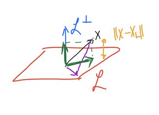
Theorem.
위 부등식의 의미는 $\mathcal{L}$ 위의 벡터와 $\mathbf{x}$ 사이의 거리를 잴 때, orthogonal proj. $\mathbf{x}_{\mathcal{L}}$이 가장 짧은 거리를 뱉음을 말한다. 그림으로 확인하면 아래와 같다.
Definition. idempotent or projection
$A \in \mathbb{R}^{n\times n}$ is called an <idempotent> or <projection> matrix if $A^2 = A$.
Theorem.
T.F.A.E.
(1) $A\mathbf{x}$ is the orthogonal projection of $\mathbf{x}$ onto $\mathcal{C}(A)$.
이 명제는 $\mathbf{x}$에 $A$를 곱하는 연산(매핑) 자체가 $\{A\mathbf{x} : \mathbf{x} \in \mathbb{R}^n \}$인 집합을 유도하는데, 이 집합이 바로 $\mathcal{C}(A)$이다.
(2) $A$ is a projection and $\mathcal{N}(A) \perp \mathcal{C}(A)$.
즉, for every $\mathbf{x} \in \mathcal{N}(A)$, $\mathbf{y} \in \mathcal{C}(A)$, $\mathbf{x}^T \mathbf{y} = 0$.
(3) $A$ is symmetric and idempotent.
그래서 만약 위의 명제 중 하나라도 성립한다면, $A$는 <orthogonal projection matrix> onto $\mathcal{C}(A)$가 된다.
Theorem.
Let $A \in \mathbb{R}^{n\times n}$ and symmetric. Then, T.F.A.E.
(1) $A^2 = A$
(2) All eigenvalues of $A$ are either 0 or 1.
(3) $\text{rank}(A) + \text{rank}(I_n - A) = n$
((1)$\implies$(2))는 쉽게 <spectral decomposition>을 활용하면, 쉽게 증명할 수 있다.
Because $A$ is symmetric, $A = UDU^T$ by spectral theorem.
By statement (1), $A^2 = A$
\[A^2 = (UDU^T)(UDU^T) = UD^2U^T = UDU^T\]따라서, $D^2 = D$. 이것을 만족하려면, $d_i^2 = d_i$가 되어야 한다. 이것은 $d_i = 0$ or $d_i = 1$일 때만 가능하다. $\blacksquare$
eigenvalue $d_i$가 0 or 1이라는 사실은 proj. $A$가 $d_i = 1$인 특정 $u_i$ 벡터만 살리게 하는 연산임을 알 수 있게 해준다.
((2)$\implies$(3))도 증명해보자. 이건 rank과 eigenvalue 사이의 관계를 통해 쉽게 증명할 수 있다.
rank는 (# of non-zero eigenvalue)로 정의된다. orthognoal proj인 $A$는 eigvenvalue가 0 또는 1이므로 $d_i = 1$의 갯수를 세면 된다.
$I_n - A$를 살펴보자. 이건 $A$의 $d_i$의 값을 토글시켜준다. 따라서, $I_n - A$의 rank는 $A$의 것과 complement하게 된다. $\text{rank}(I_n - A) = n - \text{rank}(A)$. $\blacksquare$
드디어 마지막 Theorem이다. 하지만, 아래의 명제는 이 <통계적 데이터마이닝>이라는 과목에서 <Regression>을 다룰 때 정말정말 많이 쓰게 되는 정리이므로, 정말 중요하다! 🔥
Theorem.
Let $X = (\mathbf{x}_1, \dots, \mathbf{x}_p)$ be an $n\times p$ matrix with $\text{rank}(X) = p$3 and
\[H = X(X^TX)^{-1}X^T\]Then, $H$ is the orthogonal projection onto $C(X)$, that is
(1) $H^2 = H$
(2) $\mathcal(H) \perp \mathcal{N}(H)$
(3) $\mathcal{C}(H) = \mathcal{C}(X)$
이때, $X$로부터 유도한 matrix $H$를 <hat matrix>라고 한다.