
Decision Tree
2021-1학기, 대학에서 ‘통계적 데이터마이닝’ 수업을 듣고 공부한 바를 정리한 글입니다. 지적은 언제나 환영입니다 :)
💥 이번 포스트는 <Decision Tree>를 수학적으로 정의하는 내용을 다룹니다. DT에 대한 정의와 개념은 다른 포스트를 참고해주세요 😉
DT Estimation
DT를 이루는 각 terminal node 또는 leaf node는 DT가 분할하는 region $R_i$에 대응된다.
DT는 regression과 classification 두 문제에서도 모두 적용해볼 수 있는데, 각 경우에 대한 DT estimation function $f$는 아래와 같이 정의된다.
1. DT estimation in regression problem
\[\hat{f}(x) = \sum^M_{m=1} \hat{c}_m \cdot I(x\in R_m)\]where
\[\hat{c}_m = \frac{1}{n_m} \sum_{x_i \in R_m} y_i\]$n_m$ is the # of training data in $R_m$.
그냥 terminal node에 속하는 training data의 평균으로 estimation 한다고 생각하면 된다.
2. DT estimation in classification problem
\[\hat{P}(Y=k \mid X=x) = \hat{p}_{mk} = \frac{1}{n_m} \sum_{x_i \in R_m} I(y_i = k) \quad \text{for} \quad x \in R_m\]Then, for given $X = x$, estiation $\hat{Y}$ is
\[\hat{Y} = \underset{k}{\text{argmax}} \; \hat{P}(Y=k \mid X=x)\]그냥 다수결에 의해 estimation 한다고 생각하면 된다.
DT의 장점은 좋은 interpretation power를 제공한다는 것이다! 때로는 결정에 대한 이유를 설명해야 하는 경우가 있는데, DT는 이런 상황에서 좋은 interpretation insight를 제공한다.
ex: a bank must explain reasons for rejection to a loan applicant.
DT Construction
DT는 아래 4가지 과정을 통해 만들어진다.
1. Growing
- Find an optimal splitting rule for each node and grow the tree.
- Stop growing if stopping rule is satisfied.
2. Prunning
- Remove nodes which increase prediction error or which have inappropriate inference rules.
(Complexity 감소! 😆)
※ # of terminal nodes는 DT model의 complexity에 영향을 준다.
3. Validation
- Validate to decide how much we prune the tree. (Overfitting과 관련)
4. Interpretation & Prediction
- Interpret the constructed tree & Predict!
Splitting Rule
DT를 만드는 각 과정에서, 아래 두 가지를 결정해줘야 한다.
- splitting variable $X_j$
- splitting criterion
이때, $X_j$가 continuous인지 categorical인지에 따라 criterion을 만드는 상황이 달라진다.
Splitting Rule: Regression
Assume that all input variables are continuous and
\[R_1 (j, s) = \left\{ X : X_j \le s \right\} \quad \text{and} \quad R_2(j, s) = \left\{ X : X_j > s \right\}\]splitting crieterion을 얻기 위해 splitting variable $X_j$와 split point $s$를 결정하는 문제는 아래의 식을 푸는 것과 동치다.
\[\min_{j, s} \left[ \min_{c_1} \left( \sum_{x_i \in R_1(j, s)} (y_i - c_1)^2\right) + \min_{c_2} \left( \sum_{x_i \in R_2 (j, s)} (y_i - c_2)^2 \right) \right]\]이때, $c_1$과 $c_2$는 $R_1(j, s)$와 $R_2(j, 2)$에 속하는 data에 대한 평균값이다.
위의 식을 잘 살펴보면, 결국 “training error”를 최소화하는 $X_j$와 $s$를 찾는 문제임을 볼 수 있다!
Splitting Rule: Classification
Classification도 마찬가지로 “training error”를 최소화하는 아래의 식을 풀어 splitting criterion을 구할 수 있다.
\[\min_{j, s} \left[ \min_{k_1} \left( \sum_{x_i \in R_1(j, s)} I(y_i \ne k_1) \right) + \min_{k_2} \left( \sum_{x_i \in R_2(j, s)} I(y_i \ne k_2) \right) \right]\]마찬가지로 이때, $k_1$과 $k_2$는 $R_1(j, s)$, $R_2(j, s)$에 속하는 data에서 다수결에 의해 구한 label이다.
Classification DT에서는 Splitting이 좋은지 안 좋은지 <Impurity>를 통해 측정해볼 수 있다. 그래서 위의 경우는 zero-one loss를 통해 criterion을 결정했는데, 이 방식은 곧 <misclassification error>라는 impurtiy measure를 사용한 것과 같다. 다른 impurity measure를 주어 동일한 training data라도 다른 DT를 얻을 수 있다!
Impurity Measures
1. Misclassification Error
\[\frac{1}{n_m} \sum_{i \in R_m} I(y_i \ne k_m) = 1 - \hat{p}_{mk_m}\]2. Gini Index
\[\sum^K_{k = 1} \hat{p}_{mk} (1 - \hat{p}_{mk})\]3. Cross-Entropy or Deviance
\[- \sum^K_{k=1} \hat{p}_{mk} \log \hat{p}_{mk}\]Pruning
DT는 splitting의 계속한다면, tratining error는 0으로 수렴한다. 그러나 이것은 overfitting을 야기하고, model의 generalization을 떨어뜨린다. 그래서 node이 갯수를 줄이는 pruning 과정이 필요하다.
Let $T_0$ be a large tree obtatined by splitting.
A subtree $T \subset T_0$ is any tree that can be obtained by pruning.
let $n_m = \left| \{ i : x_i \in R_m \} \right|$ and \(\displaystyle\hat{c}_m = \frac{1}{n_m} \sum_{x_i \in R_m} y_i\).
1. In a regression,
\[Q_m (T) = \frac{1}{n_m} \sum_{x_i \in R_m} (y_i - \hat{c}_m)^2\]2. In a classication (ver. Gini Index)
\[Q_m(T) = \sum^K_{k=1} \hat{p}_{mk} (1-\hat{p}_{mk})\]Then, cost complexity pruning is defined by
\[C_{\alpha}(T) = \left(\sum^{|T|}_{m=1} n_m Q_m(T)\right) + \alpha |T|\]where $\alpha > 0$ is a tuning parameter.
$C_\alpha(T)$에 대한 식을 잘 살펴보면, “training err”와 “complexity panelty”에 대한 텀이 있음을 확인할 수 있다.
이제, 위의 $C_\alpha(T)$를 기준으로 Best Pruning Subtree $T_\alpha$를 결정할 수 있다.
\[T_\alpha = \underset{T}{\text{argmin}} \; C_{\alpha} (T) \quad \text{where} \quad T \subset T_0\]위와 같은 접근법을 <weakest link pruning>라고도 한다.
tuning parameter $\alpha$는 generalization error를 최소화하는 것을 골라서 사용하면 된다고 한다. (Cross Validation을 활용하는 것 같다.)
Sensitivity & Specificity
Medical Classification Problem을 다루는 상황에서 $Y=1$이 disease state라고 가정하자. 이때, <sensitivity>와 <specificity>는 아래와 같이 정의된다.
Definition. Sensitivity
“Probability of predicting disease given true disease.”
True Positive Rate를 의미한다. 또는 <Recall>이라고 한다.
\[P(\hat{Y} = 1 \mid Y = 1)\]Definition. Specificity
“Probability of predicting non-disease given true non-disease.”
True Negative Rate를 의미한다.
\[P(\hat{Y} = 0 \mid Y = 0)\]ROC curve
앞에서 살펴본 DT는 다수결(majority vote)에 의해 prediction을 결정했다. 그러나 다수결 방식 외에도 어떤 threshold 값을 정해, spam/normal을 분류해볼 수도 있다.
\[\hat{Y} = I\left( \hat{P}(Y=1 \mid X=x) > c \right)\]for some $c > 0.5$.
이때, 우리는 classiciation rule $c$의 값을 바꿔가며, “sensitivity-specificity”를 측정할 수 있는데, 이것을 pair로 삼아 plot으로 그린 것이 바로 <ROC curve; Receiver Operating Characteristic curve>다.
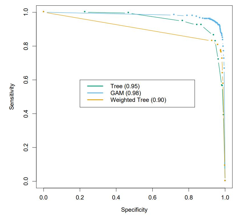
ps) ROC curve는 classification problem에서만 유도할 수 있다!
이때, ROC curve의 <AUC; Area Under the Curve>를 통해 모델의 성능을 비교 평가할 수도 있다.
DT: 장점 & 단점
Advantages.
- Robust to input outliers
- Non-parameteric model
Disadvantages.
- Poor prediction accuracy with continuous output compared to linear regression model.
- When depth is too large, not only accuracy but interpretation are bad 😥
- Heavy computation cost
- Unstable
- Absence of linearity
- Absence of Main effects: all nodes are high order interactions.
- Discontinuity
이어지는 챕터에서는 통계적 모델의 꽃🌹이라고 할 수 있는 <Boosting>에 대해 다룬다. 내용이 쉽진 않지만, 현대 통계의 핵심이기 때문에 잘 익혀둬야 하는 테크닉이다.