
Feature Selection Techniques
2021-1학기, 대학에서 ‘통계적 데이터마이닝’ 수업을 듣고 공부한 바를 정리한 글입니다. 지적은 언제나 환영입니다 :)
우리는 Feature의 차원이 늘어남에 따라 <Curse of Dimensionality>라는 문제를 갖게 된다. 이런 문제를 해결하기 위해서는 많은 기법들이 제시되었고, 이번 포스트에서는 그 기법 중 전체 feature에서 몇개를 선택해 사용하는 <Feature Selection>의 기법들에 대해 소개할 예정이다 😁
Best Subset Selection
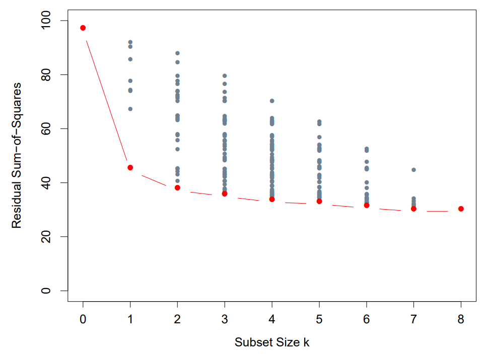
For given $k \le p$, choose $k$ input variables. This makes $\binom{n}{k}$ number of models. Find a model with which the residual mean square error is minimized among all models having $k$ input variables. Denote the model as $M_k$.
Select the optimal model among $M_0, M_1, \dots, M_p$. For $M_p$, this means we use all the input variables.
💥 이때, 어떤 모델이 좋은지는 Trainin Err가 아니라 Test Err를 봐야 한다!
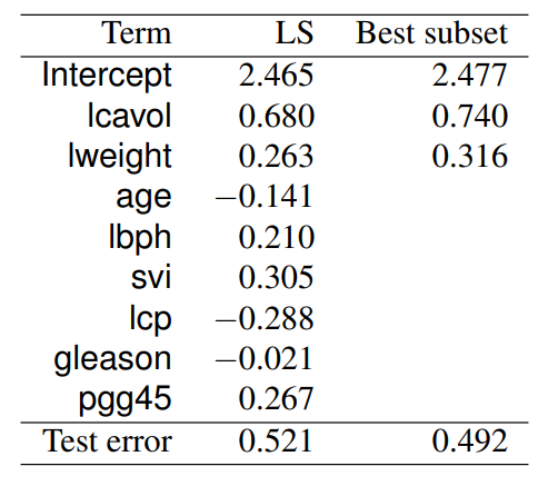
Prostate cancer dataset
<Best subset Selection>의 결과를 살펴보면, 더 적은 feature를 사용했음에도 불구하고 weight는 비슷하게 나왔고, 또 예측 성능 역시 전체 feature를 쓰는 것과 비슷한 수준으로 나왔다.
당연하게도 더 적은 feature를 썼으니 계산 측면에서도 이득! 😁
However, if $p$ is large, say $\ge 40$, it becomes computationally infeasible.
\[\binom{p}{k} = O(p^k)\]이런 계산상의 이슈 때문에 <Best Subset Selection> 대신 <Forward & Backward Selection> 기법을 사용한다.
Forward Stepwise Selection
Start with the model $M_0$ containing the intercept only.
Construct a sequence of models $M_1, \dots, M_p$ by sequentially adding the predictor that most improves the fit .
Choose the best model among $M_0, \dots, M_p$.
즉, input variable을 하나 추가할 때, Test Err가 가장 크게 낮아지는 녀석을 하나 넣겠다는 말이다!
Backward Stepwise Selection
Start with the full model $M_p$.
Construct a sequence of models $M_{p-1}, \dots, M_0$ by sequentially deleting the predictor that has the least impact on the fit.
Choose the best model among $M_p, \dots, M_0$.
즉, input variable을 하나 제거할 때, Test Err가 제일 적게 나오는 녀석을 뺀다는 말이다!
Mallow’s $C_p$
<Mallow’s $C_p$> 이하 $C_p$는 어떤 통계 모델 $M$를 평가하는 지표 중 하나다.
\[C_p (M) = \frac{1}{n} \cdot \left( \sum^n_{i=1} (y_i - \hat{y})^2 + 2d \hat{\sigma}^2 \right)\]즉, $C_p$는 Test Err와 함께 모델 피처 수 $d$를 고려한다는 말이다!
그래서 모델을 선택할 때, $C_p$가 가장 낮은 모델을 선택하면 된다.
AIC & BIC
<AIC; Akaike Information Criterion>과 <BIC; Bayesian Information Criterion>은 좀더 general한 model selection 지표이다.
<AIC> & <BIC>는 <MLE> 기법과도 관련되어 있다.
\[\text{AIC}(M) = - \frac{2}{n} \cdot \text{loglik} + \frac{2d}{n}\]이때, $\text{loglik}$는 “log-likelihood”의 약자로,<AIC>가 MLE에 의해 최대화된 “log-likelihood” 텀에 변수의 갯수 $d$에 따른 패널티를 추가한 지표를 확인할 수 있다.
피처를 많이 쓰는 모델이라면($d$가 큰) RSS는 작아지게 된다. 그러나 AIC와 BIC는 피처 수 $d$를 포함하기 때문에 AIC/BIC가 가장 작은 모델을 쓴다는 것은 우도(likelihood)를 가장 크게 하는(explainable) 동시에 피처 갯수는 가장 적은(parsimonious) 최적의 모델을 쓴다는 의미이다.
\[\text{BIC}(M) = - \frac{2}{n} \cdot \text{loglik} + \frac{d \cdot \log(n)}{n}\]<AIC>의 경우 <Mallow’s $C_p$>와 동치라고 하며, <BIC>가 <AIC>보다 더 심플한 모델을 선호한다고 한다.
Instability of Variable Selection
“Variable selection methods are known to be unstable.”
- Breiman, L. (1996)
“Unstable” means that small change of data results in large change of the estimator.
This is because variable selection uses hard decision rule (hard survivie or die rule).
<Variable Selection>의 ‘instability’ 문제에 대한 대안으로 다음 포스트에서 소개할 <Shrinkage method>를 사용할 수 있다.