PCA
2021-1학기, 대학에서 ‘통계적 데이터마이닝’ 수업을 듣고 공부한 바를 정리한 글입니다. 지적은 언제나 환영입니다 :)
Introduction to PCA
<PCA; Principal Component Analysis>는 차원축소(dimensionality reduction)에 주요한 기법으로 사용되는 테크닉이다.
✨ Goal ✨
To find low-dimensional representation of input variables which contains most information in data
Image from ‘stackoverflow’
이때, “contains most information”이란 무슨 의미일까? <PCA>에서는 이것을 데이터의 “분산(variance)”을 최대한 보존하는 것이라고 말한다! 이렇게 데이터의 분산을 보존하는 방향을 <principal component direction>라고 하며, 우리가 <PCA>를 수행하기 위해 찾아야 하는 대상이다! 😁
First Principal Component
For a design matrix $X = \left[ X_1, X_2, \dots, X_p \right]$, the first principal component $Z_1$ is the normalized linear combination:
\[Z_1 = \phi_{11} X_1 + \cdots + \phi_{1p}X_p\]that has the largest variance.
by normalization, $\sum^p_{j=1} \phi_{1j}^2 = 1$; normalization을 했기 때문에, principal component의 direction이 unique하게 정의된다.
The coefficient vector $\phi_1 = (\phi_{11}, \dots, \phi_{1p})^T$ is called the “loading vector of the first principal component”.
Q. Given a $n\times p$ design matrix $X$, how can we estimate $\phi_1$??
Let $X = (X_1, \dots, X_p)^T$, and w.o.l.g. let’s assume that $E[X] = 0$ by standardization and $\text{Var}(X) = \Sigma$.
Then, for $Z_1 = \phi_{11}X_1 + \cdots + \phi_{1p}X_p$, we want to maximuze $\text{Var}(Z_1)$!
\[\begin{aligned} \text{maximize} \; \text{Var}(Z_1) &= \underset{\phi_{11}, \dots, \phi_{1p}}{\text{maximize}} \; \text{Var}(\phi_{11}X_1 + \cdots + \phi_{1p}X_p) \\ &= \underset{\phi_{11}, \dots, \phi_{1p}}{\text{maximize}} \; \text{Var}(\phi_1^T X) \\ &= \underset{\phi_{11}, \dots, \phi_{1p}}{\text{maximize}} \; \phi_1^T \text{Var}(X) \phi_1 \\ &= \underset{\phi_{11}, \dots, \phi_{1p}}{\text{maximize}} \; \phi_1^T \Sigma \phi_1 \quad \text{s.t.} \quad \phi_{11}^2 + \cdots \phi_{1p}^2 = 1 \end{aligned}\]이때, covariance matrix $\Sigma$는 symmetric matrix이기 때문에 <spectral decomposition>이 가능하다!
\[\Sigma = UDU^T\]또, covariance matrix $\Sigma$는 positive definite matrix이다.
\[x^T \Sigma x \succ 0\]이에 따라 모든 egiven value가 positive다.
\[\Sigma = UDU^T = d_1 u_1 u_1^T + \cdots + d_p u_p u_p^T\]w.o.l.g. $0 \le d_1 \le \cdots \le d_p$.
이제 covariance matrix $\Sigma$에 대해선 충분히 살펴봤고, 이 $\Sigma$로 $\phi$를 표현해보자. 우리는 $\Sigma$의 Orthogomal matrix $U$를 사용해 아래와 같이 $\phi$를 $U$-basis expansion 할 수 있다.
\[\phi = (u_1^T\phi) u_1 + \cdots (u_p^T \phi) u_p = U \begin{pmatrix} u_1^T \phi \\ \vdots \\ u_p^T \phi \end{pmatrix}\]이때, $\phi^T \phi = 1$이기 때문에 $(u_1^T\phi)^2 + \cdots (u_p^T \phi)^2 = 1$이다.
\[\begin{aligned} \phi^T \Sigma \phi &= (u_1^T \phi, \, \dots, \, u_p^T \phi) \cancel{U^T} \cdot \cancel{U}D\cancel{U^T} \cdot \cancel{U} \begin{pmatrix} u_1^T \phi \\ \vdots \\ u_p^T \phi \end{pmatrix} \\ &= (u_1^T \phi, \, \dots, \, u_p^T \phi) D \begin{pmatrix} u_1^T \phi \\ \vdots \\ u_p^T \phi \end{pmatrix} \\ &= d_1 (u_1^T \phi)^2 + \cdots + d_p (u_p^T \phi)^2 \end{aligned}\]즉, maximum variance를 달성하기 위해 우리는 $\phi^T\Sigma \phi$를 최대로 만들어야 한다!
이때, covariance matrix $\Sigma$의 eigen value $d_i$는 통제할 수 있는 값이 아니다! 대신 가장 큰 eigen value이 $d_p$에 곱해지는 $(u_p^T \phi)^2$의 값은 조정할 수 있다!!
이때, $(u_p^T \phi)^2$의 값이 가장 커지는 경우는 바로 $\phi$가 $u_p$가 될 때이다!! ($u_p^T u_p = 1$)
즉, the constraint maximization problem for $\phi_1$의 solution은 $u_p$, the eigen vector associated with the largest eigen value $d_p$이다!
앞에서 살펴본 과정을 다시 formal하게 기술해보자!
Definition. First Principal Component
Since we are only considering variance, we may assume that each column of $X$ is centered. (컬럼 평균이 0)
Let define $z_{i1}$ to be
\[z_{i1} = \phi_{11} x_{i1} + \cdots + \phi_{1p}x_{ip} = (X\phi_1)_i\]The each $z_{i1}$ are called “the scores of the first principal component”.
Then, we can find an estimator $\hat{\phi}_1$ of $\phi_1$ by solving the following constraint maximizing problem.
\[\underset{\phi_1}{\text{maximize}} \left\{ \frac{1}{n} \sum^n_{i=1} z_{i1}^2 \right\} \quad \text{subject to} \; \sum^p_{j=1} \phi_{1j}^2 = 1\]Equivalently, $\phi_1$ can be obtained by
\[\underset{\phi_1}{\text{maximize}} \; \phi_1^T \hat{\Sigma} \phi_1 \quad \text{subject to} \; \sum^p_{j=1} \phi_{1j}^2 = 1\]where $\hat{\Sigma} = X^T X / n$, the sample covariance matrix.
Therefore, $\hat{\phi_1}$ is the eigen vector of $\hat{\Sigma}$ associated with the largest eigen value!
Second and more Principal Components
The <second principal component> $Z_2$ is the normalized linear combination of $X_1, \dots, X_p$ that has maximal variance out of all normalized linear combination that are uncorrelated with $Z_1$.
이때, <second principal component>는 $Z_1$을 구할 때처럼 아주 쉽게 구할 수 있다. 그냥 second largest eigen value에 연관된 eigen vector가 $Z_2$가 된다!! (원래 eigen vector끼리는 서로 orthogonal하다.)
$k$-th principal component에 대해서도 그냥 $k$번째 eigen value의 eigen vector를 쓰면 된다!!
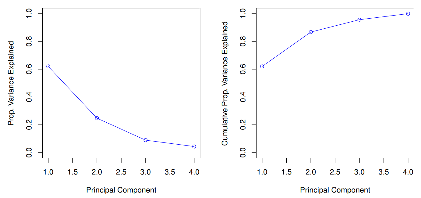
PCA Metric
<PCA>에서는 <PVE; Proportion of Variance Explained> of the m-th principal component라는 metric를 정의해 사용한다.
\[\frac{\sum^n_{i=1} z_{im}^2}{\sum^p_{j=1} \sum^n_{i=1} x_{ij}^2} = \frac{\sum^n_{i=1} z_{im}^2 / n}{\sum^p_{j=1} \sum^n_{i=1} x_{ij}^2 / n} = \frac{\text{Var}(Z_m)}{\sum^p_{j=1} \text{Var}(X_j)}\]이때, <PVE> 값을 보고, 몇개의 principal component를 사용할 것인지 결정한다!