
Supp-1: Linear Algebra - 3
2021-1학기, 대학에서 ‘통계적 데이터마이닝’ 수업을 듣고 공부한 바를 정리한 글입니다. 지적은 언제나 환영입니다 :)
Set-up
formulas.
1. $\displaystyle UU^T = \sum^n_{i=1} \mathbf{u}_i \mathbf{u}_i^T$, where $U = \left( \mathbf{u}_1, \dots, \mathbf{u}_n \right) \in \mathbb{R}^{n \times n}$
2. $\displaystyle UDU^T = \sum^n_{i=1} d_i \mathbf{u}_i \mathbf{u}_i^T$, where $D = \text{diag}(d_i)$
행렬곱을 표현하는 유용한 방식이니 익숙해지면 좋다! 앞으로 나오는 내용에서 자주 등장한다!
Definition. Orthogonal Matrix
An <orthogonal matrix> $U$ is a matrix such that $UU^T = U^TU = I_n$.
Spectral Decomposition
Theorem. Spectral Decomposition; Eigen Decomposition
For a real symmetric matrix $A \in \mathbb{R}^{n\times n}$, there exists a diagonal matrix $D = \text{diag}(d_1, \dots, d_n)$ and an orthogonal matrix $U$ s.t. $A = UDU^T$.
즉, 모든 symmetric matrix는 $UDU^T$의 형태로 decompose 가능함을 말한다!
Note.
- Each $d_i$ is an real eigenvalue of $A$.
- $\mathbf{u}_i$ is the eigenvector associated with $d_i$, where $U = \left( \mathbf{u}_1, \dots, \mathbf{u}_n \right)$.
- $\displaystyle A = UDU^T = \sum^n_{i=1} d_i \mathbf{u}_i \mathbf{u}_i^T$
<Spectral Decomposition>은 기하학적 이해가 수반되어야 한다.
먼저, orthogonal matrix $U$에 대해 $U$는 선형변환에서 일종의 rotation matrix의 역할을 한다.
\[\mathbf{x} \longrightarrow U \mathbf{x}\]이제 $A\mathbf{x}$를 해석하기 위해 $UDU^T\mathbf{x}$를 단계별로 해석해보자.
1. $U^T \mathbf{x}$; 회전을 통해 좌표축 변환
$U^T$는 회전 변환을 수행한다. 따라서, $e_1$, $e_2$ 좌표계 위에 있던 $\mathbf{x}$를 $u_1$, $u_2$ 좌표계로 회전 변환한다.
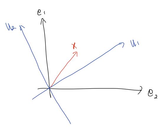
이때, $u_1$, $u_2$는 $U^T$의 각 열으로써 $A$의 eigen vector이다.
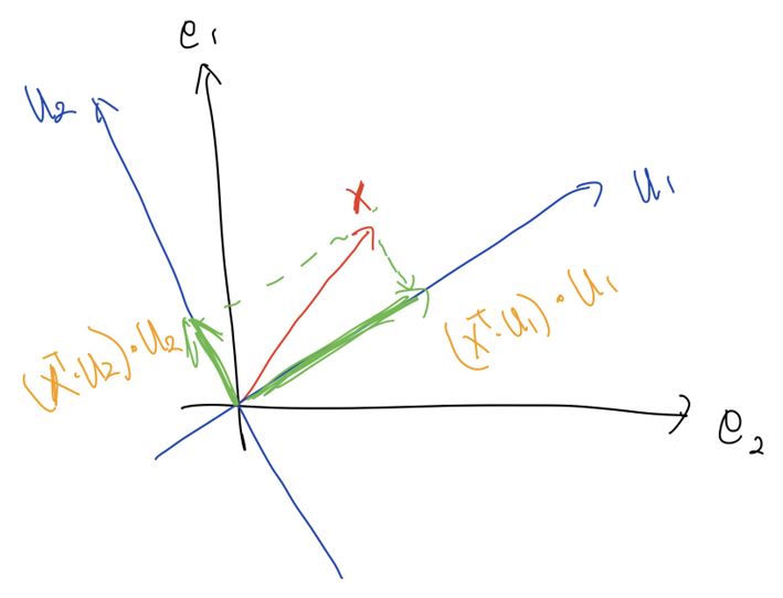
그리고 $U^T \mathbf{x}$를 계산해보면,
\[U^T \mathbf{x} = \left(u_1, u_2 \right) \cdot \mathbf{x} = \begin{pmatrix} (\mathbf{x}^T u_1) \cdot u_1 \\ (\mathbf{x}^T u_2) \cdot u_2 \end{pmatrix}\]가 되고, 이것은 $\mathbf{x}$를 $u_1$, $u_2$ 축으로 <projection>한 것과 같다.
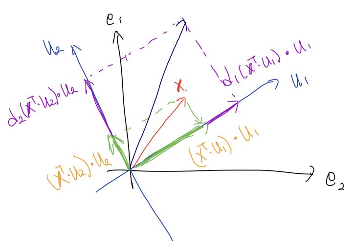
2. $D \left( U^T \mathbf{x} \right)$; 스칼라 곱
$D$는 diagnomal matrix이기 때문에 $u_1$, $u_2$ 방향의 벡터에 대한 스칼라 곱을 하는 역할이다.
3. $U \left( D U^T \mathbf{x} \right)$; 원래의 좌표축으로 역-회전
마지막으로 처음에 곱한 $U^T$의 역-회전 변환인 $U$를 적용해 다시 $e_1$, $e_2$의 좌표계로 되돌려 준다.
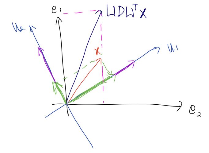
그래서 식을 정리하면, 아래와 같다.
\[UDU^T \mathbf{x} = UD \begin{pmatrix} u_1^T \mathbf{x} \\ \vdots \\ u_n^T \mathbf{x} \end{pmatrix} = U \begin{pmatrix} d_1 u_1^T \mathbf{x} \\ \vdots \\ d_n u_n^T \mathbf{x} \end{pmatrix} = d_1 u_1 u_1^T \mathbf{x} + \cdots + d_n u_n u_n^T \mathbf{x}\]Singular Value Decomposition
<Sepctral Theorem>은 대칭 행렬에 대해서 기술한 정리였다. 이것을 일반적인 형태의 행렬로 일반화한 것이 바로 <특이값 분해 Singular Value Decomposition>이다. 😎
Theorem. Singular Value Decomposition
For any $n \times p$ matrix $A$, there exist matrices $U \in \mathbb{R}^{n\times n}$, $D \in \mathbb{R}^{n\times p}$, and $V \in \mathbb{R}^{p\times p}$ s.t.
\[A = UDV^T\]where
- $D = \text{diag}(d_1, \dots, d_p)$ with $d_i \ge 0$
- $d_j$s are called <singular value> of $A$.
- $U$ is an orthogonal matrix from $AA^T = U(\Sigma\Sigma^T)U^T$
- $V$ is an orthogonal matrix from $A^T A = V(\Sigma^T \Sigma)V^T$
Low Rank Approximation
SVD를 잘 이용하면, 행렬 $A$에 대한 <Low Rank Approximation> $A_k$를 유도할 수 있다.
Let $A = UDV^T$ and assume that $n \gg p$, then
\[A = \begin{bmatrix} \vert & & \vert \\ \mathbf{u}_1 & \cdots & \mathbf{u}_n \\ \vert & & \vert \\ \end{bmatrix} \begin{bmatrix} d_1 & & \\ & \ddots \\ & & d_p \\ & O & \end{bmatrix} \begin{bmatrix} - & \mathbf{v}_1^T & - \\ & \vdots & \\ - & \mathbf{v}_p^T & - \\ \end{bmatrix} = d_1 \mathbf{u}_1 \mathbf{v}_1^T + \cdots + d_p \mathbf{u}_p \mathbf{v}_p^T\]이때, 표기의 편의를 위해 singular value $d_i$에 대해 descending order로 표기를 한다.
\[\text{where} \quad d_1 \ge d_2 \cdots \ge d_p\]주목할 점은 식의 우변의 $\mathbf{u}_i \mathbf{v}_i^T$은 rank-1 matrix라는 점이다. 즉, SVD를 하게 되면 행렬 $A$를 rank-1의 matrix로 분해한 것이 된다.
이제 위의 결과를 가지고 Approximation $A_k$를 유도할 수 있다.
\[A_k = \begin{bmatrix} \vert & & \vert \\ \mathbf{u}_1 & \cdots & \mathbf{u}_k \\ \vert & & \vert \\ \end{bmatrix} \begin{bmatrix} d_1 & & \\ & \ddots & \\ & & d_k \\ & O & \end{bmatrix} \begin{bmatrix} - & \mathbf{v}_1^T & - \\ & \vdots & \\ - & \mathbf{v}_k^T & - \\ \end{bmatrix} = d_1 \mathbf{u}_1 \mathbf{v}_1^T + \cdots + d_k \mathbf{u}_k \mathbf{v}_k^T\]즉, $A_k$는 $A$를 SVD로 분해해 표현한 것에서 앞의 $k$개의 rank-1 matrix를 모은 것이다! 우리가 $d_i$를 내림차순으로 정렬해 표현했기 때문에, 뒤로 갈수록 작은 $d_j$를 얻게 되어 있다. 그래서 $A_k$는 앞의 $k$개 $d_i$만을 선택해 $A$를 근사한 것이다!
이때, <Low Rank Approximation>의 error는 아래와 같이 <Frobenius norm>으로 정의한다.
\[\begin{aligned} \| A - A_k \|^2_F &= \text{tr}\left( (A-A_k)^T (A-A_k) \right) \\ &= d_{k+1}^2 + d_{k+2}^2 + \cdots + d_p^2 \end{aligned}\]그래서, 만약 뒷부분의 $d_{k+1}, \cdots d_p$의 크기가 작다면, Low Rank Approx는 충분히 정확한 근사를 수행함을 보장할 수 있다!!
ps. 이런 Low Rank Approx는 생각보다 자주 사용되는 기법이라고 한다.
ps. Netflix의 추천 알고리즘 Contest에서 이 SVD를 활용해 Low Rank Approx를 하는 추천 알고리즘을 구현한 팀이 우승을 차지했다고 한다.
지금까지 행렬을 분해하는 두 가지 방법인 <Spectral Decomposition>과 <Singular Value Decomposition>를 살펴봤다. 이 두 개념은 이어지는 내용인 행렬의 <Nonnegative Definite>, <Positive Definite>를 정의할 때 바탕이 된다.