
Regression Spline
2021-1학기, 대학에서 ‘통계적 데이터마이닝’ 수업을 듣고 공부한 바를 정리한 글입니다. 지적은 언제나 환영입니다 :)
이전 챕터에서는 parameter를 추론해 linear regreeion & linear classification을 수행하는 방법을 살펴보았다.
\[f(x) = E[Y \mid X = x] = \beta^T x\]이번 챕터에서는 non-linear model에 대해 살펴볼 예정이며, <Basis Expansion>과 <Kernel Method>을 중심으로 non-linear model을 살펴본다!
Basis Expansion
Definition. Basis expansion
For $m=1, \dots, M$, let $h_m: \mathbb{R}^p \rightarrow \mathbb{R}$ be the $m$-th transformation of $X$.
Then, we model as
\[f(X) = \sum^M_{m=1} \beta_m h_m (X)\]with a linear basis expansion in $X$.
Example.
1. 1-dimensional projection
\[h_m(X) = X_m \quad \text{for} \quad m=1, \dots, p\]2. Covariatic transform (정식 명칭은 아니고, Cov 같은 느낌이라 본인은 이렇게 부른다.)
\[h_m (X) = X^2_j \quad \text{or} \quad h_m(X) = X_j X_k\]3. log transform or root transform
\[h_m(X) = \log (X_j) \quad \text{of} \quad h_m (X) = \sqrt{X_j}\]4. range transform
\[h_m(X) = I(L_m \le X_k < U_m)\]특정 범위에 따라 $X_k$를 제단하는 transform이다.
5. Splines 🔥
곧 만날 예정!
6. Wavelet bases
정말 중요하게 쓰이는 방법이지만, 정규 수업에서는 다루지 않았다.
Polynomial Regression
-- Weierstrass's Approximation Theorem
For $p$-dimensional $X$, the $m$-th order polynomial is given as
\[f(X) = \beta_0 + \left(\sum^p_{j=1} \beta_j X_j\right) + \left(\sum^{p^2}_{j,k} \beta_{jk} X_j X_k\right) + \cdots + \left(\sum^{p^m}_{j_1, \dots, j_m} \beta_{j_1, \dots, j_m} X_{j_1} \cdots X_{jm} \right)\]- As $p$ increases, the # of parameters grows exponentially.
- In general, it is difficult to estimate $p$-dimensional regression function for large $p$.
그리고 그런 $m$-th order polynomial 방식은 <Multi-collinearity>에 대한 문제도 가지고 있다. 👇
논의의 편의를 위해 $p=1$라고 하자. 그리고, $X_i$를 아래와 같이 디자인 하자.
Let $X_1 \sim \text{Unif}(0, 1)$, and $X_m = X_1^m$ for $m \le 4$.
이때, $X_1, \dots, X_4$의 Corr를 구해보면,
\[\text{Corr}(X_1, \dots, X_4) = \begin{bmatrix} 1.00 & 0.97 & 0.92 & 0.86 \\ 0.97 & 1.00 & 0.98 & 0.95 \\ 0.92 & 0.98 & 1.00 & 0.99 \\ 0.86 & 0.95 & 0.99 & 1.00 \end{bmatrix}\]와 같은데, Corr의 값을 살펴보면, 모두 1에 가까운 값을 가진다. 이것은 각 독립변수 사이에 강한 상관관계가 있다는 것을 의미하며, 이것을 <Multi-collinearity; 다중공선성>이라고 한다.
- High order polynomials are often unstable at the boundary.
→ bad!!! 😥
<Polynomial Regression>에서의 문제를 해결하기 위해 함수를 local로 분할해 근사하는 <Local Polynomial Regression> 방식이 제안 되었다.
Local Polynomial Regression
-- Talyor's Theorem
Supp. that $p=1$. Divide domain interval $(a, b)$ into $K+1$ sub-intervals $(a=\xi_0, \xi_1], (\xi_1, \xi_2], \dots, (\xi_k , b=\xi_{k+1})$.
Then, a local polynomial regression model is given as
\[f(X) = \sum^{K+1}_{i=1} f_{i}(X) \cdot I(\xi_{i-1} < X \le \xi_i)\]where $f_i$ are polynomials and $\xi_i$ are the knots.
앞에서 살펴본 <Polynomial Regression>과 비교했을 때, 범위 전체를 도메인으로 갖는 polynomial을 취하는 것이 아니라 domain interval을 분할해 polynomial fitting을 한다는 점이 다르다.
Example. Constant & Linear
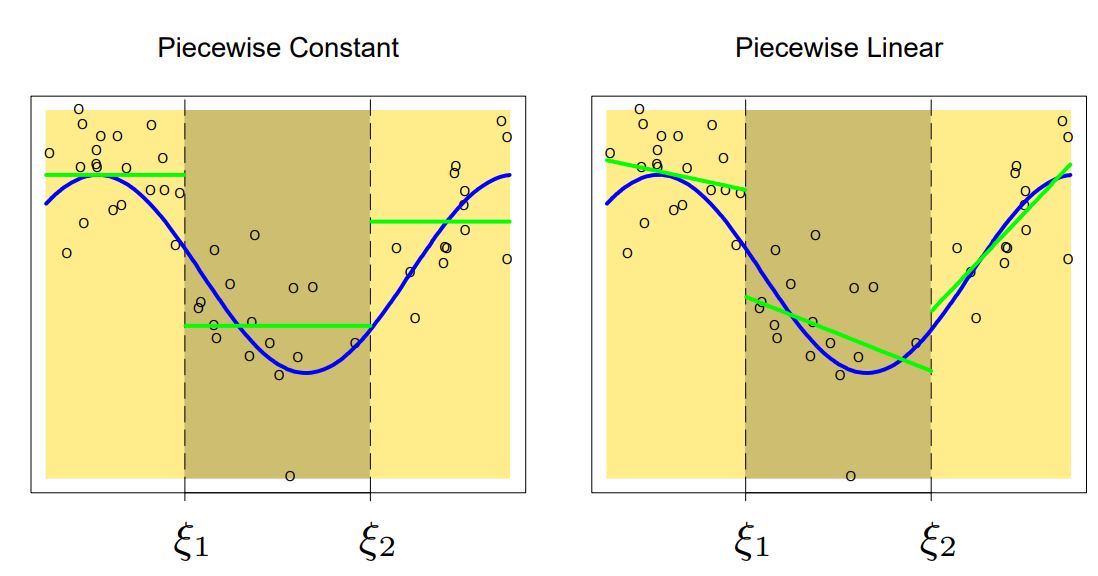
$f_i$를 constant function, linear function으로 모델링 했을 때의 결과이다. 그림에서도 볼 수 있듯이 knots 주변에서 continuous 하지 않다. 이걸 non-continuous 현상은 order가 커져도 여전히 발생한다. 😥
<Regression Spline>은 <Local Polynomial Regression>에 “continuous & continuous derivative에 대한 제약”을 주어 non-continuous 문제를 해결한다!
Regression Spine
Definition. Regression Polynomial Spline
Given a fixed knot sequence $\xi_1, \dots, \xi_K$,, a function defined on an open interval $(a, b)$ is called a <regression (polynomial) spline of order $M$> if it is a piecewise polynomial of order $M$ on each of the intervals.
\[(a=\xi_0, \xi_1], (\xi_1, \xi_2], \dots, (\xi_k , b=\xi_{k+1})\]and has continuous derivatives up to order $(M-1)$.
앞에서 살펴본 <Local Polynomial Regression>의 not-continuous 문제를 해결하기 위해 <Regression Spline>에서는 piecewise polynomial이 $(M-1)$차 연속인 도함수를 가져야 한다는 조건이 추가된 것이다!!
Example. 3rd-order polynomial ($M=3$)
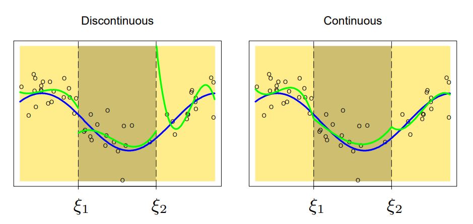
왼쪽은 앞에서 살펴본 <Local polynomial regression>의 모델이다. knot에서 not-continuous하다.
오른쪽은 knot에서 continuous해야 한다는 제약을 준 모델이다.
이는 $x \mapsto a_3 x^3 + a_x x^3 + a_1 x + a_0$인 각 $f_i\left((\xi_{i-1}, \xi_i]\right)$에 대해
\[f_i(\xi_i) = f_{i+1}(\xi_i)\]라는 조건이 추가된 것이다. 이는 곧, $f_i(\xi_i) = f_{i+1}(\xi_i)$이기 때문에, $f_{i+1}$에서 $b_4, b_3, b_2$에 대한 값이 정해졌다면, 자동으로 $b_0$의 값이 결정된다.
\[a_3 x^3 + a_2 x^2 + a_1 x + a_0 = b_3 x^3 + b_2 x^2 + b_1 x + \cancelto{\text{calculated by constraint}}{b_0}\]따라서, estimate 해야 하는 Coefficients의 갯수는
\[(M+1)(K+1) - (K-1)\](ex: If $M=3$ and $K=2$, then we need to estimate $4 + 4 - 1$ coefficients.)
Example. 3rd-order polynomial with 1st & 2nd derivative
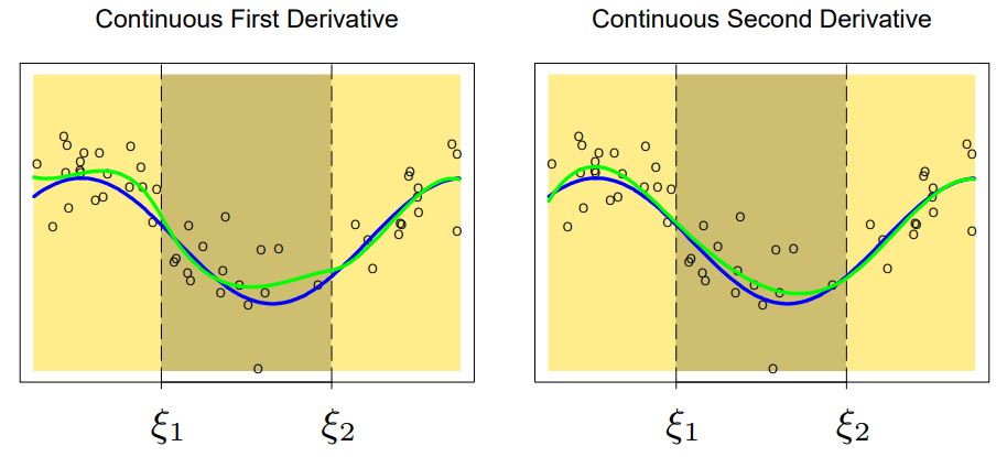
이번에는 “knot에서 continuous” 조건과 함께 “knot에서 1st/2nd derivatives continuous” 조건이 추가되었다.
이를 만족하려면, $f_i’ (\xi_i) = f_{i+1}’(\xi_i)$를 만족해야 하며, 이것은 곧
\[3 a_3 x^2 + 2 a_2 x + a_1 = 3 b_3 x^2 + 2 b_2 x + \cancelto{\text{calculated by constraint}}{b_1}\]이므로 constraint를 통해 $b_1$의 값을 정할 수 있다는 말이 된다. 2nd derivative continuous에 대해서도 동일한 방법으로 접근하면 된다.
따라서, estimate 해야 하는 Coefficients의 갯수는
\[(M+1)(K+1) - MK = M + K + 1\]Spline basis function
Notation.
또는
\[(x-\xi)_{+}^M = \begin{cases} (x-\xi)^M & \text{if} \quad x > \xi \\ 0 & \text{else} \end{cases}\]Example.
만약 $M=1$(linear) and $K=2$라면, spline basis function은 아래와 같다.
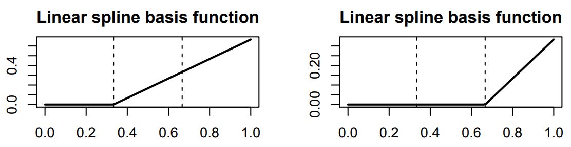
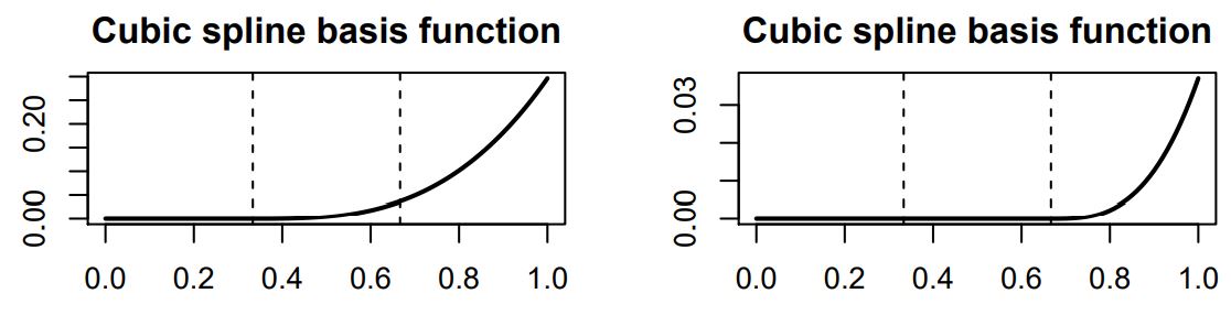
만약 $M=3$(cubic) and $K=2$라면, spline basis function은 아래와 같다.
Natural Cubic Spline
완벽할 것 같은 <Regression Spline> 방식도 작은 문제를 가지고 있다. 바로 양끝 boundary에서 regression이 잘 안 된다는 것이다. 이를 해결하기 위해 <Natural cubic spline>은 양끝에서 linear로 모델링 한다.
Definition. Natural Cubic Spline
A cubic spline is called a <natural cubic spline>, if it is linear beyond the boundary knots $\xi_1$ and $\xi_K$.

(출처: Stanford - STAT202)
그림에서 볼 수 있듯이 높은 차원의 $M$으로 근사할 수록 <Regression Spline>은 boundary에서 성능이 저하되는 걸 볼 수 있다. <Natural Cubic Spline>은 양끝에서 linear로 근사함으로써 이 문제를 해결한다!
<Natural Cubic Spline>에서 estimate 해야 하는 Coefficient 수는 $M=3$이므로
\[(M + K + 1) - (2 \times 2) = (3 + K + 1) - 4 = K\]Smoothing Splines
<knot selection>은 Spline Method의 주된 이슈이다. <smoothing spline>은 이 문제를 아래와 같이 해결한다!
Consider $\hat{f} = \underset{f\in\mathcal{F}}{\text{argmin}} \; \text{RSS}_{\lambda}(f)$, where
\[\text{RSS}_{\lambda} \; (f) = \left(\sum^n_{i=1} \left\{ y_i - f(x_i)\right\}^2\right) + \lambda \int \left\{ f''(t) \right\}^2 \; dt\]and $\lambda$ is a fixed smoothing parameter.
위의 식을 잘 살펴보면, RSS 식에 패널티 텀이 있는 것을 볼 수 있다. 이때, 패널티 텀에서는 $f’'(t)$를 적분하는데, 이것은 함수 $f(t)$에 대한 <곡률; curverture>를 의미한다. $(f’'(t))^2$는 곡률의 절댓값이며, 따라서 패널티 텀은 함수 $f(t)$가 얼마나 flunctuation이 심한지를 측정하는 텀이라고 볼 수 있다.
위의 최적화 문제의 solution인 $\hat{f}$를 <smoothing spline estimator>라고 한다!
1. If $\lambda = 0$,
then $\hat{f}$ can be any function that interpolates the data.
2. If $\lambda = \infty$,
then $\hat{f}$ is the least square estimator. (왜냐하면, $f’'(t)=0$이 되려면, $f(t)$가 linear function이어야 한다!)
3. (general case) small $\lambda$
model complexity $\uparrow$ / bias $\downarrow$ / variance $\uparrow$
(= flunctuation이 심해짐!)
4. (general case) large $\lambda$
model complexity $\downarrow$ / bias $\uparrow$ / variance $\downarrow$
만약 $\mathcal{F}$가 특정 <Sobolev space>에 속하는 어떤 함수라면, smooth spline이 곧 natural cubic spline이 된다고 한다.
ESL, Exercise 5.7
앞에서 살펴본 Smoothing Spline에 대한 식은 infinite-dimensional problem이었다 이것을 linear fit 방식으로 해결할 수도 있는데, 그 식은 아래와 같다.
\[f(\theta; x) = \sum^n_{j=1} \theta_j N_j (x)\]where $N_j$ are basis functions of natural cubic splines.
Then,
\[\text{RSS}_{\lambda} \; (\theta) = (\mathbf{y} - \mathbf{N}\theta)^T (\mathbf{y} - \mathbf{N}\theta) + \lambda \cdot \theta^T \mathbf{\Omega} \theta\]where \(\mathbf{N}_{ij} = N_j(x_i)\) and $\displaystyle\mathbf{\Omega}_{ij} = \int {N_i}’' (t) {N_j}’'(t) \; dt$.
식이 조금 복잡해보이지만, 위에서 제시한 $f(\theta; x)$를 smoothing spline의 식에 맞게 기술한 것일 뿐이다!
위의 $\text{RSS}_{\lambda}(\theta)$를 구하는 것은 그냥 $\theta$로 미분해서 최소가 되는 $\theta$를 구해주면 된다.
\[\hat{f}(x) = \sum^n_{j=1} \hat{\theta}_j N_j(x)\]where
\[\hat{\theta} = (\mathbf{N}^T \mathbf{N} + \lambda \mathbf{\Omega})^{-1}\mathbf{N}^T \mathbf{y}\]내부에 regularization 텀으로 인해 $\lambda \mathbf{\Omega}$가 생겼다!
이어지는 포스트에서는 spline method의 남은 내용을 좀더 살펴본다. 🤩