
Clustering
2021-1학기, 대학에서 ‘통계적 데이터마이닝’ 수업을 듣고 공부한 바를 정리한 글입니다. 지적은 언제나 환영입니다 :)
“Clustering refers to a braod set of techniques for partitioning a dataset into homogeneous subgroups called clusters.”
✨ How can we define the “homogeneity”?
이번 포스트에서 우리는 “clustering”을 수행하는 3가지 방식에 대해 살펴볼 것이다.
- Distance-based clustering
- Hierarchical clustering
- Model-based clustering
K-means clustering
Algorithm for partitiong a dataset into $k$ subgroups.
이때, number of cluster $K$는 미리 정해져야 함! (HOW?)
<K-means>에서 우리는 <within-cluster variation measure>를 정의해 사용한다!!
For a set $C \subset \{ 1, 2, \dots, n\}$, the within-cluster variation measure $W(C)$ is
\[W(C) = \frac{1}{\left| C \right|} \sum_{\begin{aligned} i, j &\in C \\ i &< j \end{aligned}} \left\| x_i - x_j \right\|_2^2\]※ small value of $W(C)$ may represent a good cluster.
즉, <within-cluster variation>은 cluster 내에서의 variance를 측정하는 지표인 것이다!
우리가 데이터를 $C_1, \dots, C_K$의 집합으로 분할한다면, 이것은 아래의 최적화 문제를 푸는 것과 같다.
\[\underset{C_1, \dots, C_K}{\text{minimize}} \left\{ \sum_{k=1}^K W(C_k) \right\}\]Algorithm. Brute Force
나이브하게 접근해보자면, $n$개 데이터를 $K$개 부분집합으로 분할하는 가짓수는 $K^n$이다. 즉, 나이브한 접근은 exponential complexity가 걸리는 아주 어려운 문제다 ㅠㅠ
그래서 Brute Force와 같은 방식이 아니라, 위 문제의 sub-optimal solution을 찾는 방식으로 <K-means clustering>을 수행한다!
Algorithm. K-means Algorithm
1. Randomly partition $\{1, \dots, n \}$ into $K$ clusters.
2. Repeat the following until converges.
- For each cluster, compute the cluster centroid.
- Assign each obs to the cluster whose centroid is the closest.
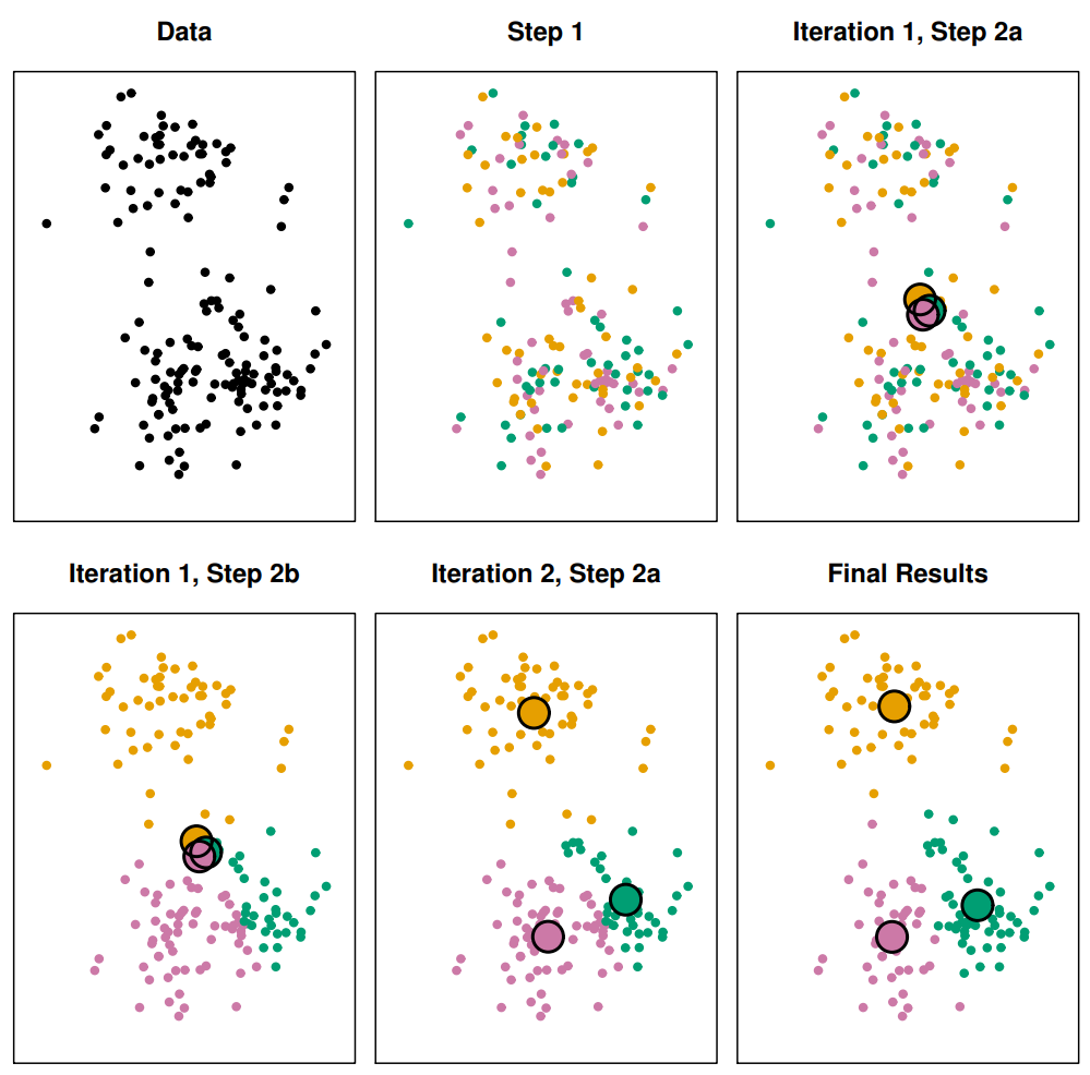
figure from ISLR
그림을 보면, 2번만에 수렴한 것을 볼 수 있다!!
✨ NOTE: <K-means algorithm> is guaranteed to decrease $W(C)$ because
\[W(C_k) = \frac{1}{\left| C \right|} \sum_{\begin{aligned} i, j &\in C \\ i &< j \end{aligned}} \left\| x_i - x_j \right\|_2^2 = \sum_{i \in C_k} \left\| x_i - \bar{x}_k \right\|_2^2\]where $\bar{x}_k$ is mean of cluster $C_k$.
식 유도
추후에 업데이트!
<K-means algorithm>은 global optimum이 아니라 local optimum을 찾는 것으로 알려져 있다.
<K-means algorithm>의 결과는 initial cluster에 따라 바뀌기 때문에, 서로 다른 몇가지 initial cluster로 여려번 돌려보는 것이 권장된다.
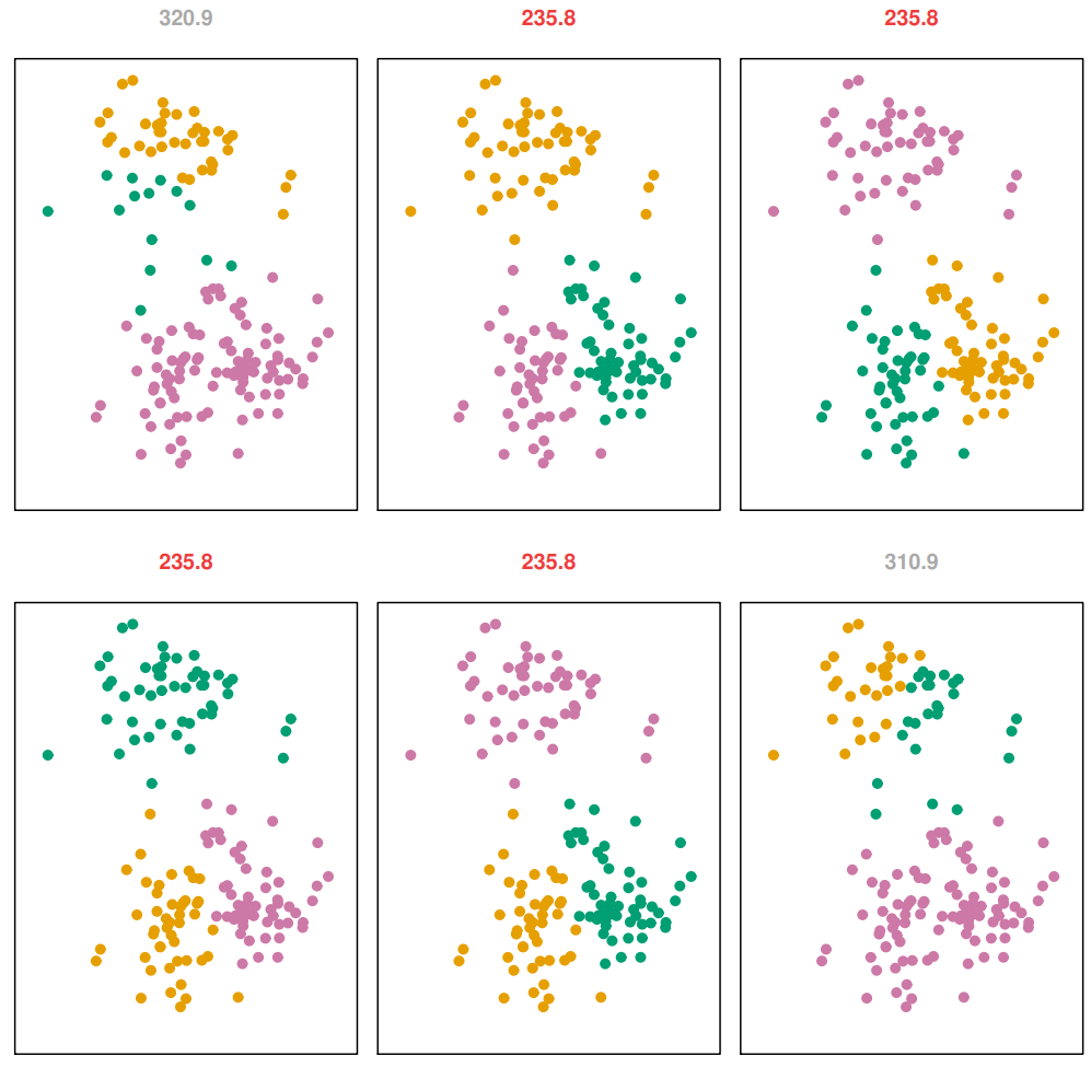
figure from ISLR
그림을 보면, 하나의 형태로 cluster가 결정되는 것이 아니다.
위 그림에서는 2, 3, 4, 5번째의 경우로 clustering 되는 것이 우세하다.
Hierarchical Clustering
<Hierarchical Clustering>에서는 “dendrogram”이라는 것을 통해 cluster를 나누고, 또 그 계층을 분석한다.
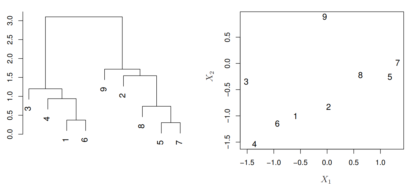
figure from ISLR
위 그림을 바탕으로 어떻게 <Hierarchical Clustering>을 수행하고, “dendrogram”을 만드는지 살펴보자.
먼저, 위의 2차원 데이터 분포에서 가장 가까운 두 점을 찾는다. 여기서는 (5, 7)이다. 두 점을 왼쪽의 dendrogram에 표시하고, 두 점을 하나의 cluster로 묶는다. cluster 하나가 추가된 데이터 분포에서 또 가장 가까운 두 점을 찾는다. 여기서는 (1, 6)이다. 이 두 점을 왼쪽의 dendrogram에 표시하고, 또 하나의 cluster로 묶는다. 또 진행하면, 이번에는 ((5, 7), 8)이 가장 가까운 쌍이다. 이것을 왼쪽의 dendrogram에 표시한다. … (continue) …
방법은 정말 간단하다!! 하지만, 여기서도 몇가지 이슈가 있다. 그것은 바로 “cluster-point 거리를 어떻게 측정할 것인가”다!
두 ‘점’의 거리를 측정하는 것은 간단하게 유클리드 거리로 측정할 수 있다.
그러나 cluster-point, cluster-cluster의 거리를 측정하는 것은 여러가지 방법이 가능하다.
- Complete linkage: maximal intercluster dissimilarity
- Single linkage: minimal intercluster dissimilarity
- Average linkage: mean intercluster dissimilarity
- Centroid linkage: dissimilarity between the centroids
보통 “complete linkage”와 “average linkage”를 사용한다. “centroid linkage”의 경우, 순서가 역전되는 경우가 발생하기 때문에, 권장하진 않는다.
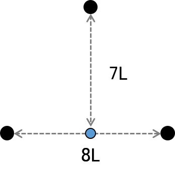
Cluster 사이 거리는 non-decreasing 해야 하는데, 이 경우는 8L 다음에 7L이 되어 inversion이 생겼다.
Spectral Clustering
💥 정말 특이한 Clustering 방식이다. 내용이 조금 어려우니 집중하자!
Traditional clustering (ex. K-means) does not work well when clusters are non-convex. <Spectral Clustering> is designed for these situations.
일단 바빠서 패-스
이번 포스트에서 살펴본 방식은 모두 휴리스틱 방법들이다. 이어지는 포스트에서는 모델(model)을 기반으로 하는 <Model-based clustering>을 살펴본다. <Mixture Model>, <EM-Algorithm> 등 무시무시한 것들이 왕창 나온다;;