
Predictive Distribution
“Machine Learning”을 공부하면서 개인적인 용도로 정리한 포스트입니다. 지적은 언제나 환영입니다 :)
기획 시리즈: Bayesian Regression
Bayesian Approach
이번 포스트부터 본격적으로 Bayesian Approach에 대해 탐구한다. 먼저 Bayesian의 관점에서는 확률(probability)을 “가설에 대한 믿음의 정도”로서 이해한다. 그래서 사전 믿음을 가지고 가설을 살펴보고, 이후에 데이터를 관측했다면 그 데이터를 가지고 새롭게 믿음을 갱신해 사후 믿음을 얻는다. 이런 수집-갱신의 과정을 데이터가 발생할 때마다 계속 반복한다.
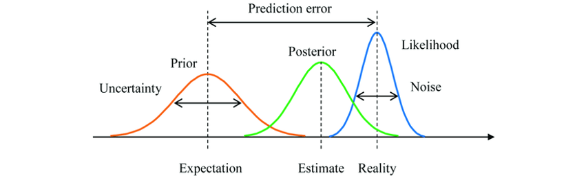
기억할 점은 Bayesian Approach는 항상 ‘불확실성(uncertainty)’에 대해 얘기한다는 것이다. 고전적인 확률론이 Point Estimation으로 unbiased estimator 또는 the most efficient estimator of $\theta$1를 구하거나 또는 Interval Estimation으로 confidence level을 구하는 등의 추정을 수행하지만, Bayesian Approach는 parameter $\theta$에 대한 ‘확률 분포’를 찾는 것을 목표로 한다. 그래서 Point Estimation에서 처럼 parameter의 값을 $\theta = \theta_0$로 특정하는 것이 아니라 “$\mu = 4$, $\sigma^2 = 1$인 정규분포로 parameter가 분포되어 있다”라고 말한다.
Bayesian Approach에서는 관측 데이터가 추가됨에 따라 parameter의 distribution을 계속 갱신한다. 이는 parameter의 prior distribution을 새롭게 관측된 데이터로 갱신해 posterior distribution을 얻는 셈이다. 이 아티클에서는 이것을 “데이터가 확률 분포를 잡아당기는 자석과 같다”고 표현하는데, 표현이 그럴싸 하다 😲 자세한 내용은 해당 아티클의 요 부분을 잠깐 읽어보고 오는 걸 추천한다. 글을 통해 데이터가 posterior distribution을 어떻게 갱신하는지 그리고 prior distribution을 잘 잡는게 중요한 이유를 깨달을 수 있다 👍
기존의 고전적인 방법은 Point Estimator나 confidence interval를 유도했다. 그러나 Bayesian Approach에서는 그런 것들이 전혀 없으며👋 단지 parameter에 대한 posterior distribution을 이용해 새로운 데이터 $x^{*}$를 예측할 뿐이다. 그리고 이 과정에서 등장하는 것이 바로 <Predictive Distribution; 예측 분포>이다!
Parameter Posterior
앞의 문단에서 Bayesian Approach가 관측 데이터로 parameter의 distribution을 갱신한다고 기술했다. 이것을 좀더 살펴보자! 제일 먼저 parameter $\theta$에 대한 prior distribution을 가정한다. 이것을 <prior distribution of parameter> 또는 <parameter prior>라고 하며, 여기서는 아래와 같은 정규 분포를 가정하겠다.
\[\theta \sim N(0, \tau^2 I)\]이제 관측된 데이터 $X = \{ x^{(1)}, \dots, x^{(m)} \}$를 이용해 <parameter prior> $p(\theta)$를 갱신해보자. <parameter posterior> $p(\theta \mid X)$는 Bayes Rule에 따라 아래와 같이 유도할 수 있다.
\[\begin{aligned} p(\theta \mid X) &= \frac{p(X \mid \theta) p(\theta)}{p(X)} = \frac{p(X \mid \theta) p(\theta)}{\int_{\theta'} p(X \mid \theta') p(\theta') d\theta'} \\ &= \frac{p(\theta) \prod^m_{i=1} p(x^{(i)} \mid \theta)}{\int_{\theta'} p(\theta') \prod^m_{i=1} p(x^{(i)} \mid \theta') d\theta'} \end{aligned}\]이때, likelihood의 $p(x^{(i)} \mid \theta)$는 $\theta$로 parameterized된 확률 변수 $X$에 대한 확률 분포로 이항 분포, 정규 분포, 포아송 분포 등등이 가능하다. likelihood는 데이터가 parameter $\theta$에 의해 어떻게 parameterized 되어 있을 것이라고 가정하는 것이기 때문에 갱신하는 대상이 아니다! 🙌
이항분포
\[p(x^{(i)} \mid \theta) = \frac{n!}{x!(n-x)!} \theta^x (1 - \theta)^{(n-x)}\]1D-정규분포
\[p(x^{(i)} \mid \theta) = \frac{1}{\sqrt{2\pi} \sigma} \exp \left( - \frac{(x^{(i)} - \theta)^2}{2\sigma^2}\right)\]2D-정규분포 ($x^{(i)} \in \mathbb{R}^2$, also $\theta \in \mathbb{R}^2$)
\[p(x^{(i)} \mid \theta) = \frac{1}{\sqrt{2\pi} \sigma} \exp \left( - \frac{(x^{(i)} - \theta)^2}{2\sigma^2}\right)\]등등등!!
Example. Parameter Posterior
동전을 던졌을 때, 앞면이 나올 확률이 균일 분포를 따른다. 동전을 던졌더니 앞면이 나왔을 때, parameter poster를 구하라.
Solution
“앞면이 나올 확률이 균일 분포를 따른다.”
→ $p(\theta) = I_{(0 \le \theta \le 1)}$ (parameter prior)
“동전을 던진다.”
→ $p(x \mid \theta) = \theta^x (1 - \theta)^{(1-x)}$ (likelihood)
“동전을 던졌더니 앞면이 나왔을 때”
→ $x_1 = 1$
갱신된 parameter posterior에서는 앞면이 많이 나올 거라는 확률(=믿음)이 반영되었다.
$\blacksquare$
Predictive Distribution
<Predictive Distribution; 예측 분포>는 unobserved data $x^{*} \in X^{*}$에 대한 prediction을 수행하는 과정에서 유도하는 분포이다. 그래서 이름에 “predictive”라는 이름이 붙었다고 할 수 있다. 뇌피셜입니다 <Predictive Distribution>은 parameter prior로 유도하는지, observed data $X$가 반영된 parameter posterior로 유도하는지에 따라 두 가지로 나뉜다.
Definition. Prior Predictive Distribution
Let $X = \{ x^{(1)}, \dots, x^{(m)} \}$ be a set of observed data, $X^{*}$ be a set of unobsersed data, and $x^{*} \in X^{*}$.
Then, the <prior predictive distribution> is
\[p(x^{*}) = \int p(x^{*}, \theta) d\theta = \int p(x^{*} \mid \theta) p(\theta) d\theta\]즉, likelihood $p(x \mid \theta)$를 parameter prior $p(\theta)$의 확률 분포를 고려해 적분한 것이 <prior predictive distribution>이다.
그러나 <prior predictive distribution>은 observed data $X$를 전혀 쓰고 있지 않다. observed data를 제대로 활용하려면 parameter posterior $p(\theta \mid X)$로 유도한 <posterior predictive distribution>을 사용해야 한다!
Definition. Posterior Predictive Distribution
보통 $x^{*}$와 $X$를 독립이라고 가정하기 때문에 또는 iid를 가정하므로,
\[p(x^{*} \mid X) = \int p(x^{*} \mid \theta, X) p(\theta \mid X) d\theta = \int p(x^{*} \mid \theta) p(\theta \mid X) d\theta\]<prior predictive distribution>과 비교했을 때 달라진 점은 적분 내부의 함수가 parameter prior $p(\theta)$에서 parameter posterior $p(\theta \mid X)$로 바뀌었다는 점이다! <posterior predictive distribution>은 관측된 데이터로 갱신된 <parameter posterior>를 사용했기 때문에 실제 모수(parameter)와 근접할 것으로 기대되는 분포를 바탕으로 예측(prediction)했다고 기대하게 된다.
이 아티클의 해당 부분에서 predictive distribution을 유도하는 간단한 예제를 풀어볼 수 있다. 문제가 좋으니 한번쯤 풀어보도록 하자 👀 참고로 첫번째 예제에서 Gamma function $\Gamma$를 써서 적분하는 부분은 Beta Distribution에 대한 적분이다.
다음 포스트에서는 <Predictive Distribution>을 이용해 Regression Problem을 다룬다. 이것을 <Bayesian Linear Regression>이라고 하며 이번 포스트를 잘 이해했다면 다음 포스트를 쉽게 이해할 수 있을 것이다 😁
reference
- [번역] 선형 회귀 모델 Bayesians vs Frequentists
- Prior & Posterior Predictive Distributions
- 사전예측분포와 사후예측분포(Prior and posterior predictive distribution)
- [Bayesian DL] 1. Properties of Gaussian Distribution and Prior(Posterior) Predictive Distribution
-
unbiased estimaor with the smallest variance ↩