
Bayesian Regression
“Machine Learning”을 공부하면서 개인적인 용도로 정리한 포스트입니다. 지적은 언제나 환영입니다 :)
기획 시리즈: Bayesian Regression
Bayesian Linear Regression
이번 포스트에서는 앞에서 다룬 <parameter posterior>, <posterior predictive distribution>을 Regression Problem에 적용한다. 사실 <Bayesian Linear Regression>은 단순히 <posterior predictive distribution under the regression problem>일 뿐이다! 🙌
관측된 데이터 $S = (X, y)$가 존재해 이것으로 <parameter prior>를 갱신해보자. Bayes Rule에 따르면 아래와 같이 <parameter posterior>를 유도할 수 있다.
\[\begin{aligned} p(\theta \mid S) &= \frac{p(S \mid \theta) p(\theta)}{p(S)} = \frac{p(S \mid \theta) p(\theta)}{\int_{\theta'} p(S \mid \theta') p(\theta') d\theta'} \\ &= \frac{p(\theta) \prod^m_{i=1} p(y^{(i)} \mid x^{(i)}, \theta)}{\int_{\theta'} p(\theta') \prod^m_{i=1} p(y^{(i)} \mid x^{(i)}, \theta') d\theta'} \end{aligned}\]이때, likelihood의 $p(y^{(i)} \mid x^{(i)}, \theta)$ 텀은 아래와 같이 기술할 수 있다.
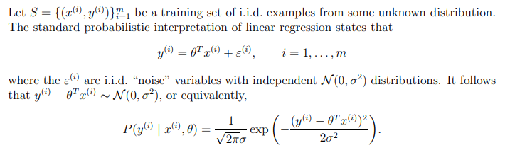
\[p(y^{(i)} \mid x^{(i)}, \theta) = \frac{1}{\sqrt{2\pi} \sigma} \exp \left( - \frac{(y^{(i)} - \theta^T x^{(i)})^2}{2\sigma^2}\right)\]이것은 아래와 같은 regression의 가정을 통해 유도된 것으로 $y$를 하나의 확률 변수로 취급한다는 의미를 가진다. 또한, 이전 포스트에서는 likelihood function이 이항 분포, 정규 분포 등등의 분포를 가질 수 있었는데, regression problem의 상황에서는 likelihood를 Gaussian distribution로 설정할 수 밖에 없다! 🙌
이번에는 Regression problem에 대한 <Predictive Distribution>을 살펴보자. observed data $S = (X, y)$(train-set)와 unobserved data $S^{*} = (X^{*}, y^{*})$(test-set)가 있을 때, unobserved data $x^{*} \in X^{*}$에 대한 prediction을 수행하는 과정에서 유도하는 분포이다.
Definition. Prior Predictive Distribution (Regression)
Let $S = \{ (X, y) \}$ be a set of observed data, $X^{*}$ be a set of unobsersed data, and $x^{*} \in X^{*}$.
Then, the <prior predictive distribution> is
\[p(y^{*} \mid x^{*}) = \int p(y^{*}, \theta \mid x^{*}) d\theta = \int p(y^{*} \mid x^{*}, \theta) p(\theta) d\theta\]그러나 <prior predictive distribution>은 observed data $S$를 전혀 쓰고 있지 않다. observed data를 제대로 활용하려면 parameter posterior $p(\theta \mid S)$로 유도한 <posterior predictive distribution>을 사용해야 한다!
Definition. Posterior Predictive Distribution (Regression)
보통 $x^{*}$와 $S$를 독립이라고 가정하기 때문에 또는 iid를 가정하므로,
\[p(y^{*} \mid x^{*}, S) = \int p(y^{*} \mid x^{*}, S, \theta) p(\theta \mid S) d\theta = \int p(y^{*} \mid x^{*}, \theta) p(\theta \mid S) d\theta\]일반적으로 regression problem에서 정의한 parameter poster $p(\theta \mid S)$와 posterior predictive distribution $p(y^{*} \mid x^{*}, S)$는 적분 계산이 매우 어렵다. 그래서 근사를 이용해 문제를 해결하는데, 시리즈의 맨 처음에 다뤘던 MAP(Maximum a Posterior)도 이런 근사 방식 중 하나이다.
다행인 점은 <Bayesian Linear Regression>은 $p(\theta \mid S)$와 $p(y^{*} \mid x^{*}, S)$에 대한 분포해가 알려져 있으며 아래와 같다.
\[\begin{aligned} \theta \mid S &\sim \mathcal{N} \left( \frac{1}{\sigma^2} A^{-1}X^T\vec{y}, \; A^{-1}\right) \\ y^{*} \mid x^{*}, S &\sim \mathcal{N} \left( \frac{1}{\sigma^2} {x^{*}}^T A^{-1} X^{T} \vec{y}, \; {x^{*}}^T A^{-1} x^{*} + \sigma^2 \right) \end{aligned}\]where $A = \frac{1}{\sigma^2}X^TX + \frac{1}{\tau^2}I$.
위의 식이 어떻게 유도 되는지는 아직 본인도 제대로 이해하지 못해서 추후에 별도의 포스트로 유도 과정을 기술하도록 하겠다 🙌
그래도 위의 식을 통해 parameter posterior와 posterior predictive distribution이 Gaussian distribution을 따른다는 것을 알 수 있으며, 특히 prediction $y^{*}$, $y^{*} = \theta^T x^{*} + \epsilon^{*}$에 대한 uncertainty와 parameter $\theta$의 선택에 대한 uncertainty도 두 식의 variance 값을 통해 확인할 수 있다! 👍
맺음말
이번 포스트를 마지막으로 Bayesian Approach 시리즈가 끝이 났다. 용어에 ‘Bayesian’이라는 말이 들어가면 어렵게만 느껴졌는데, 이번 시리즈를 통해 조금은 Bayesian Theory를 극복한 것 같다 🙌
<Bayesian Regression>이 bayesian parameteric regression이라면, bayesian regression이지만 non-parameteric model인 <Gaussian Process Regression>도 있다. 궁금하다면, 해당 포스트를 방문해보자 👏