Divergence and Curl

복수전공하고 있는 수학과의 졸업시험을 위해 학부 수학 과목들을 다시 공부하고 있습니다. 미적분학 포스트 전체 보기

어쩌면 지금 이 상태일지도…

드디어!! 미적2의 꽃이라고 할 수 있는 발산(Divergence)과 회전(Curl)이다!! 두 개념 모두 벡터장을 유체의 흐름이라고 보고, 그 유체가 한 점에 대해 팽창/압축 하고 있는지, 아니면 한 점에서 유체가 얼마나 빠르게 회전하고 있는지를 측정하는 지표이다. 🌊

Divergence

If $\mathbf{F} = P \, \mathbf{i} + Q \, \mathbf{j} + R \, \mathbf{k}$ is a vector field on $\mathbb{R}^3$,

and the below partial derivatives exist

\[\frac{\partial P}{\partial x} \text{ , } \frac{\partial Q}{\partial y} \text{ , } \frac{\partial R}{\partial z}\]

then the “divergence of $\mathbf{F}$” is a scalar value defined by

\[\text{div } \mathbf{F} = \frac{\partial P}{\partial x} + \frac{\partial Q}{\partial y} + \frac{\partial R}{\partial z}\]

발산(divergence)는 벡터장에 대해 정의하는 스칼라 함수이다. Gradient Vector $\nabla$와의 내적으로 식을 더 쉽게 표현할 수 있다.

\[\text{div } \mathbf{F} = \nabla \cdot \mathbf{F}\]

Geometric meaning

벡터장을 유체의 흐름 속이라고 표현한다면, 발산(div)는 한 점 $(x, y, z)$에 모이는(압축) 방향으로 유체가 흐르는지, 아니면 점에서 나가는(팽창)하는 방향으로 유체가 흐르는지를 수치화 하는 값이다.

• $\text{div }\mathbf{F} > 0$
  • 한 점에서 유체가 팽창한다: outflowing-ness.
• $\text{div }\mathbf{F} < 0$
  • 한 점에서 유체가 압축된다: inflowing-ness.
• $\text{div }\mathbf{F} = 0$
  • 한 점이 유체에 전혀 압력을 받고 있지 않다: incompressible.

발산에 대한 식을 3차원 공간에 대한 것으로 적었지만, 2차원 평면에서 정의한 벡터장에 대해서도 발산(divergence) 값을 계산할 수 있다.

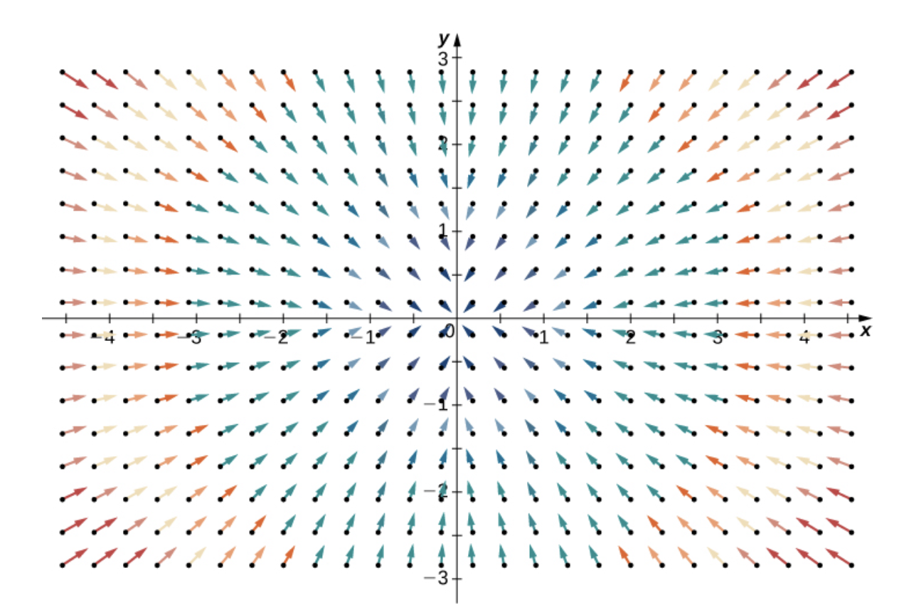Gilbert Strang - Calculus Vol 3.: Negative Divergence

위의 벡터장은 $\mathbf{F}(x, y) = \left<-y, x\right>$로 div를 계산해보면, $-2$가 된다. 따라서 모든 점이 압축하는 방향으로 압력을 받는다.

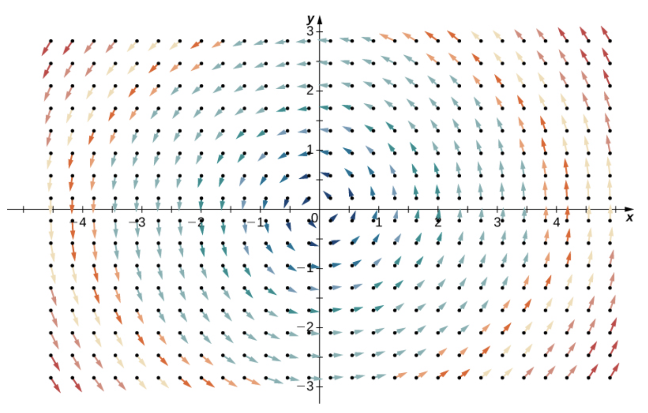Gilbert Strang - Calculus Vol 3.: Zero Divergence

반면에 압축을 전혀 받지 않는 벡터장도 있다. $\mathbf{F}(x, y) = \left<-x, y\right>$인 벡터장은 div를 계산해보면 $0$이 된다. 따라서 모든 점에서 압축을 받지 않는다.

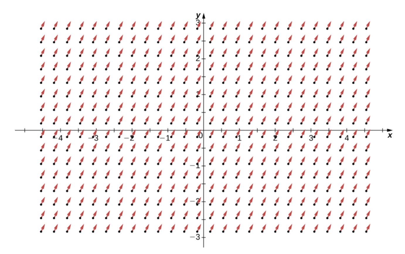Gilbert Strang - Calculus Vol 3.: Zero Divergence

또, 위와 같이 유체의 흐름이 상수인 경우도 유체가 받는 압력이 $0$으로 계산된다.

뭔가 $\text{div } \mathbf{F} = 0$인 상황을 “유체가 받는 압력이 $0$”이다 라고 표현하면 좀 모호한 감이 있다. 그래서 이렇게 표현하는 것도 가능하다.

한 지점에서 유체의 유출이나 유입되는 유량이 없다.

즉, 유체가 나가는 만큼, 어딘가에서 유체가 들어와 나가는 량을 상쇄시킨다는 것이다.

Source-free Field

위에서 설명한 것과 같이 어떤 지점 또는 영역에서 유출량이 $0$인 벡터장을 “source-free Vector Field“라고 한다. 이런 벡터장은 아무 닫힌 곡선을 잡더라도, 그 곡선에 대해 유입/유출하는 유체량이 동일하다.

“source”라는 표현은 한 점에서 나가는 유량을 말한다. 반대로 “sink”는 한 점으로 들어오는 유량을 말한다. wikipedia

또, 이런 $\text{div }\mathbf{F} = 0$인 벡터장을 “Solenoidal Vector Field“라고도 부른다. 솔레노이드는 고등학교 물리시간에 봤던 그 ‘솔레노이드’를 말한다 ㅋㅋ

Curl

If $\mathbf{F} = P \, \mathbf{i} + Q \, \mathbf{j} + R \, \mathbf{k}$ is a vector field on $\mathbb{R}^3$, and the partial derivatives of $P$, $Q$ and $R$ all exists,

then the “curl of $\mathbf{F}$” is the vector field on $\mathbb{R}^3$ defined by

\[\text{curl } \mathbf{F} = \left( \frac{\partial R}{\partial y} - \frac{\partial Q}{\partial z} \right) \mathbf{i} + \left( \frac{\partial P}{\partial z} - \frac{\partial R}{\partial x} \right) \mathbf{j} + \left( \frac{\partial Q}{\partial x} - \frac{\partial P}{\partial y} \right) \mathbf{k}\]

식이 조금 복잡한데, 위의 식을 외우기 보다는 외적으로 표기한 아래의 식으로 이해하는게 더 유용하다.

\[\text{curl } \mathbf{F} = \nabla \times \mathbf{F}\]

즉, Gradient 벡터와 벡터장을 외적한 것이 회전(curl)이다.

\[\nabla \times \mathbf{F} = \left| \begin{matrix} \mathbf{i} & \mathbf{j} & \mathbf{k} \\ \frac{\partial}{\partial x} & \frac{\partial}{\partial y} & \frac{\partial}{\partial z} \\ P & Q & R \end{matrix} \right|\]

Geometric meaning

벡터장을 유체의 흐름 속이라고 표현한다면, 회전(curl)은 한 점 $(x, y, z)$ 주변을 회전하는 유체의 회전 흐름을 표현하는 벡터다.

• curl 벡터의 방향 = 회전축
• curl 벡터의 부호 = 회전 방향: CCW(+), CW(-)
• curl 벡터의 크기 = 회전하는 속도

Gilbert Strang - Calculus Vol 3.: Zero Divergence, Positive Curl

$\mathbf{F} = \left< -y, x, 0\right>$라는 벡터장의 원점 $O$에서의 curl을 계산해보면,

\[\text{curl } \mathbf{F} = 0 \, \mathbf{i} + 0 \, \mathbf{j} + 2 \, \mathbf{k}\]

로, $+z$ 방향의 curl 벡터를 얻으며, 유체가 원점을 기준으로 시계 방향으로 회전하고 있음을 할 수 있다.

curl 벡터가 영벡터인 경우를 유체가 해당 점 주변을 회전하지 않는(irrotational)하다고 말한다. 이것은 유체가 회전 운동에서 자유롭다는 것으로, 유체가 직선 운동을 하고 있다면, 그 방향이 거의 바뀌지 않을 것임을 말한다.

Gilbert Strang - Calculus Vol 3.: Zero Divergence, Zero Curl

요런 벡터장도 curl 벡터가 영벡터인데, 유체가 움직이는 방향과 다른 방향으로 움직이게 하려는 외력이 존재하지 않기 때문이다.

If Conservative field, curl is zero vector

If $f$ a function of three variables that has continuous second-order derivatives, then

\[\text{curl}(\nabla f) = \mathbf{0}\]

정리에서는 potential function $f(x, y, z)$를 기준으로 되어 있지만, Conservative field $\mathbf{F} = \nabla f$의 경우, curl이 영벡터임을 말하고 있다.

증명은 Conservative Field의 정의에 충실하게 식을 전개하기만 하면 된다.

\[\mathbf{F} = \nabla f = \frac{\partial f}{\partial x} \, \mathbf{i} + \frac{\partial f}{\partial y} \, \mathbf{j} + \frac{\partial f}{\partial z} \, \mathbf{k}\] \[\text{curl } \mathbf{F} = \left(\frac{\partial^2 f}{\partial y\partial z} - \frac{\partial^2 f}{\partial z\partial y}\right) \, \mathbf{i} + \left(\frac{\partial^2 f}{\partial z\partial x} - \frac{\partial^2 f}{\partial x\partial z}\right) \, \mathbf{j} + \left(\frac{\partial^2 f}{\partial x\partial y} - \frac{\partial^2 f}{\partial y\partial x}\right) \, \mathbf{k} = \mathbf{0}\]

EzEz $\blacksquare$ (요게 가능한 이유는 편미분 순서를 바꿔도 상관 없다는 클레로의 정리(Clairaut’s Theorem) 때문.)

위의 정리는 Conservative 벡터장의 curl 벡터가 항상 영벡터라 계산할 필요 없다는 것도 말해주지만, 오히려 벡터장의 curl이 영벡터가 아닌 상황에서 유용하다. 왜냐하면, 대우 명제에 따라 $\text{curl }\mathbf{F} \ne 0$라면, 벡터장이 non-conservative이기 때문이다.

위의 정리의 역명제는 성립하지 않는다. $\text{curl } \mathbf{F} = \mathbf{0}$이더라도 그 벡터장이 conservative가 아닌 반례가 있기 때문.

단, 벡터장이 아래의 조건을 만족한다면 역명제도 성립한다고 한다.

If given vector field $\mathbf{F}$ is

• defined on all of $\mathbb{R}^3$
• and whose component functions have continuous partial derivatives
• and $\text{curl } \mathbf{F} = \mathbf{0}$

then $\mathbf{F}$ is a conservative vector field.

그래서 벡터 함수가 불연속성을 가지거나, 성분 함수의 편미분이 불연속성을 갖는 그런 특수한 상황만 아니라면, $\text{curl } \mathbf{F} = \mathbf{0}$인지 확인하여 conservative 여부를 판단할 수 있을 것이다 ㅎㅎ

사실 정의역이 $\mathbb{R}^3$일 필욘 없고, simply-connected region이기만 하면 된다고 한다. (증명은 이후에 스토스크 정리 할 때 배운다고 함.)

Curl and Div

어떤 벡터장에 Curl을 적용한 후, Divergence를 적용하면 재밌는 결과가 나온다.

If $\mathbf{F} = P \, \mathbf{i} + Q \, \mathbf{j} + R \, \mathbf{k}$ is a vector field on $\mathbb{R}^3$ and $p$, $Q$, and $R$ have continuous second-order partial derivatives, then

\[\text{div } \text{curl } \mathbf{F} = 0\]

증명은 curl와 div의 정의에 맞에 아래 식을 전개하면 된다. Ez

\[\text{div } \text{curl } \mathbf{F} = \nabla \cdot (\nabla \times \mathbf{F}) = 0\]

요 정리는 벡터장이 curl 연산으로 인해 만들어진 것이라면, 그것의 div가 0임을 말한다. 이것의 대우 명제를 활용하면, 어떤 벡터장 $\mathbf{G}$가 $\text{div } \mathbf{G} \ne 0$라면, 그 벡터장은 curl 벡터로 유도된 것이 아니라고 판단할 수 있다.

Vector Potential

벡터장에 curl을 적용하면 회전 벡터장이라는 또다른 벡터장이 뛰쳐나온다. 그래서 주어진 벡터장이 회전 벡터장이라면, curl을 적용한 원본 벡터장을 “Vector Potential”라고 부른다.

The vector field $\mathbf{A}$ is said to be a “vector potential” for the vector field $\mathbf{B}$ if

\[\mathbf{B} = \nabla \times \mathbf{A}\]

위의 Curl-Div 항등식을 Vector Potential로 다시 기술하면 아래와 같다.

If there exists a vector potential for the vector field $\mathbf{B}$, then

\[\nabla \cdot \mathbf{B} = 0\]

앞에 나왔던 $\nabla \times \mathbf{F} = 0$ 케이스와 좀 헷갈릴 수도 있어서 정리를 좀 해보자.

For a vector field $\mathbf{F}$

• If scalar Potential(= potential function) exists, then
  • the field is a conservative field
  • $\nabla \times \mathbf{F} = \mathbf{0}$
• If vector Potential exists, then
  • the field is a curl vector field
  • $\nabla \cdot \mathbf{F} = 0$

Vector Potential이든 Scalar Potential이든 어떤 벡터장의 원본이 되는 vector/scalar function라는게 공통점!

이때, 회전 벡터장 $\mathbf{B}$를 만드는 Vector Potential은 유일하게 결정되지 않는다.

임의의 스칼라 함수 $\psi$에 대해 아래의 등식이 성립한다.

\[\mathbf{B} = \nabla \times \mathbf{A} = \nabla \times (\mathbf{A} + \nabla \psi)\]

이것이 가능한 이유는 $\nabla \times \nabla \psi = \mathbf{0}$이기 때문이다. $\mathbf{A}$와 $\mathbf{A} + \nabla \psi$ 둘다 회전 벡터장 $\mathbf{B}$를 유도하므로, 둘다 Vector Potential 이고, Vector Potential은 유일하게 결정되지 않고 무한히 많다.

따라서, 아래의 따름 정리가 성립하는데,

If the vector field $\mathbf{B}$ has a vector potential,

then, there is a vector potential $\mathbf{A}$ for $\mathbf{B}$ with $\mathbf{A}_3 = 0$.

즉, 회전 벡터장의 Vector Potential로 $\mathbf{k}$ 컴포넌트가 0인 벡터장이 항상 존재한다는 것이다. 이 결과는 $\mathbf{k}$ 컴포넌트가 아니라 $\mathbf{i}$나 $\mathbf{j}$가 0이어도 성립한다.

Laplace Operator

벡터장 $\mathbf{F}$가 Conservative Field라면,

\[\mathbf{F} = \nabla f\]

인데, 여기에 div 연산을 한번더 수행해보자.[* curl 연산을 하면, 영벡터가 되었다: $\nabla \times \nabla f = \mathbf{0}$] 그러면 식은 아래와 같이 potential function $f$에 성분별로 편미분을 두 번 적용한 것의 합으로 표현된다.

\[\text{div}(\nabla f) = \nabla \cdot (\nabla f) = \frac{\partial^2 f}{\partial x^2} + \frac{\partial^2 f}{\partial y^2} + \frac{\partial^2 f}{\partial z^2}\]

요렇게 potential function에 Gradient 연산과 Div 연산을 연속해 수행하는 것을 간단하게 아래의 표기로 표현한다.

\[\nabla^2 f = \nabla \cdot (\nabla f) = \text{div}(\nabla f)\]

요 연산을 수행하는 연산자를 “Laplace Operator“라고 부른다. 왜냐하면, Laplace Equation에서 유래한 것이기 때문.

\[\nabla^2 f = \frac{\partial^2 f}{\partial x^2} + \frac{\partial^2 f}{\partial y^2} + \frac{\partial^2 f}{\partial z^2} = 0\]

참고로 라플라스 방정식은 미방 때 많이 볼 예정… ^^ 1학년 미적분학에서는 전혀 사용하지 않을 연산자이니 그냥 여기에서 개념만 보고 넘어갑시다!

Vector form of Green’s Theorem

그린 정리를 발산과 회전의 표기를 사용해 표현할 수도 있습니다!

포스트의 내용이 길어져서 해당 내용은 별도의 포스트로 분리하였습니다 ^^

➡️ Vector form of Green’s Theorem