
Distribution over functions & Gaussian Process
“Machine Learning”을 공부하면서 개인적인 용도로 정리한 포스트입니다. 지적은 언제나 환영입니다 :)
본 글을 읽기 전에 “Random Process“에 대한 글을 먼저 읽고 올 것을 권합니다 😉
기획 시리즈: Gaussian Process Regression
Introduction to Gaussian Process
먼저 <Gaussian distribution>을 복습해보자.
1. 1D Gaussian Distribution
\[f(x) = \frac{1}{\sqrt{2\pi} \sigma} \exp \left( - \frac{(x-\mu)^2}{2\sigma^2}\right)\]2. 2D Gaussian Distribution
\[f(\mathbf{x}) = \frac{1}{2\pi \left| \Sigma \right|^{1/2}} \exp \left( - \frac{1}{2} (\mathbf{x} - \mu)^T \Sigma^{-1} (\mathbf{x} - \mu) \right)\]3. Multi-variate Gaussian Distribution
Distribution over random vectors!
\[f(\mathbf{x}) = \frac{1}{(2\pi)^{n/2} \left| \Sigma \right|^{1/2}} \exp \left( - \frac{1}{2} (\mathbf{x} - \mu)^T \Sigma^{-1} (\mathbf{x} - \mu) \right)\]이제 <Gaussian Process>의 정의를 살펴보자.
Definition. Gaussian Process
A sequence of Gaussian distributions! <Gaussian Process> is a generlization of multi-variate Gaussian distribution. It is a distribution over random functions!
\[\mathcal{GP} (m(x), k(x, x'))\]위의 정의만 봐서는 <Gaussian Process>가 뭔지 잘 이해가 안 된다 😥 먼저 “distribution over random functions”라는 표현부터 이해해보자. <random function>이라는 낯선 개념이 등장했는데 <random variable>과는 다른 것일까?
Definition. random function
Let $\mathcal{H}$ be a class of functions mapping $\mathcal{X} \rightarrow \mathcal{Y}$. A random function $h(\cdot)$ from $\mathcal{H}$ is a function which is randomly drawn from $\mathcal{H}$, according to some probability distribution over $\mathcal{H}$.
Once a random function $h(\cdot)$ is selected from $\mathcal{H}$ probabilistically, it implies a deterministic mapping from inputs in $\mathcal{X}$ to outputs in $\mathcal{Y}$.
위에서 정의한 <random function>은 단순히 random number를 출력하는 함수가 아니다! 👊
Probability distribution over functions with finite domains
먼저 확률 분포가 어떻게 함수 위에서 정의되는지 알기 위해 $\mathcal{X}$가 finite set인 간단한 상황부터 살펴보자.
Let $\mathcal{X} = \{x_1, \dots, x_m\}$ be any finite set of elements. Now consider the set $\mathcal{H}$ of all possible functions mapping from $\mathcal{X}$ to $\mathbb{R}$.
Since the domain of any $h(\cdot) \in \mathcal{H}$ has only finite $m$ elts, we can represent $h(\cdot)$ as an $m$-dimensional vector, $\vec{h} = [h(x_1), \dots, h(x_m)]^T$.
In order to specify a probability distribution over functions $h(\cdot)$, we must associate some ‘probability density’ with each function in $\mathcal{H}$. Note that we’ve represent function $h(\cdot)$ as a vector $\vec{h}$. Then we can give a prob. distribution like gaussian as follows
\[\vec{h} \sim \mathcal{N} \left( \vec{\mu}, \; \sigma^2 I \right)\]Boom! this implies a prob. distribution over functions $h(\cdot)$, whose probability density function is given by
\[p(h) = \prod^m_{i=1} \frac{1}{\sqrt{2\pi} \sigma} \exp \left( - \frac{1}{2\sigma^2} (h(x_i) - \mu_i)^2 \right)\]위의 finite domain의 예시를 통해 우리는 prob. distribution over functions with finite domains가 finite-dimensional multi-variate Gaussian으로 표현됨을 알 수 있다! 😲 여기서 function domain $\mathcal{X}$를 infinite dimension으로 확장하면, 우리는 <Gaussian Process>를 얻게 된다! 💪
Probability distribution over functions with infinite domains
이번에는 $\mathcal{X}$에서 추출한 collection을 이용해 random variable의 집합 $\{ h(x) : x \in \mathcal{X}\}_m$를 정의해보자. $h(\cdot)$가 probabilistic 하게 결정되는 random function이기 때문에 $h(x)$도 random variable 이다. 😉 이때 domain set $\mathcal{X}$에 대해 별도로 특정하지는 않았다. 이전과 같은 finite domain을 생각해도 좋고, $\mathbb{R}$와 같은 infinite dimension을 생각해도 좋다.
우리는 finite collection of random variable $\{ h(x) : x \in \mathcal{X}\}_m$로 multi-variate Gaussian distribution을 정의할 수 있다. 이때, $\mathcal{X}$를 domain으로 갖는 $m(x)$와 $k(x, x’)$는 mean function, covariance function을 아래와 같이 정의할 수 있을 것이다.
\[\begin{aligned} m(x) &= E \left[h(x)\right] \\ k(x, x') &= E \left[ (h(x) - m(x)) (h(x') - m(x'))\right] \end{aligned}\]따라서 collection of random variable $\{ h(x) : x \in \mathcal{X}\}_m$ 위에서의 multi-variate Gaussian distribution은 아래와 같다.
\[\vec{h}_m = \begin{bmatrix} h(x_1) \\ \vdots \\ h(x_m) \end{bmatrix} \sim \mathcal{N} \left( \begin{bmatrix} m(x_1) \\ \vdots \\ m(x_m) \end{bmatrix} ,\; \begin{bmatrix} k(x_1, x_1) & \dots & k(x_1, x_m) \\ \vdots & \ddots & \vdots \\ k(x_m, x_1) & \dots & k(x_m, x_m) \end{bmatrix} \right)\]<Gaussian Process>의 정의를 다시 떠올려보자.
“A Gaussian process is a stochastic process s.t. any finite subcollection of random variables has a multivariate Gaussian distribution.”
Boom! 우리가 위에서 정의한 domain $\mathcal{X}$에서 추출한 collection of random variable $\{ h(x) : x \in \mathcal{X}\}_m$로 적절한 multi-variate Gaussian distribution을 만드는 과정은 사실 <Gaussian Process>의 정의를 재현하는 것이었다! finite collection에서 유도한 위의 표현을 일반화하면 <Gaussian Process>를 아래와 같이 적을 수 있다.
\[h(\cdot) \sim \mathcal{GP} (m(\cdot), \; k(\cdot, \cdot))\]finite domain에서 $h(x)$를 finite random vector로 이해한 것처럼, infinite domain에서의 $h(x)$는 infinite random vector로 이해할 수 있다! 🙌
mean & convariance function for GP
이제 GP가 distribution over random function이라는 점, 그리고 distribution over infinite random vector라는 것을 이해했다. 우리의 다음 관심사는 GP를 an function $m(x)$과 covariance function $k(x, x’)$이다 🙌 사실 앞의 문단에서 $m(x)$와 $k(x, x’)$의 정의를 적긴 했다만, $h(\cdot)$가 random function이기 때문에 위의 정의를 가지고는 $m(x)$, $k(x, x’)$가 정확히 어떤 함수인지 감을 잡을 순 없었을 것이다.
일반적으로 mean function $m(x)$는 어떤 real-valued function도 가능하다. 그러나 covariance function $k(x, x’)$는 GP를 marginalization 했을 때 유도되는 Covariance Matrix가 semi-positive definite 같은 covariance의 성질들을 만족해야 한다.
For covariance function $k(x, x’)$ and for any set of elts $x_1, \dots, x_m \in \mathcal{X}$, the resulting covariance matrix must be satisfy the properties of covariance matrix.
\[K = \begin{bmatrix} k(x_1, x_1) & \dots & k(x_1, x_m) \\ \vdots & \ddots & \vdots \\ k(x_m, x_1) & \dots & k(x_m, x_m) \end{bmatrix}\]For example, all $k(x, x’) \ge 0$ and $K$ is a non-negative definite matrix.
위의 조건을 보면 유효한 $k(x, x’)$를 찾는 것은 까마득해 보인다 😥 그.러.나. Chuong B. Do의 아티클에 따르면 valid convariance function에 대한 조건이 곧 <Mercer’s theorem; 머서의 정리>에서 요구하는 kernel의 조건과 동일하다고 말한다! 😲 그래서 <Mercer’s theorem>이 보장하는 valid kernel function $k(x, x’)$를 사용하면 convariance의 성질을 고민하지 않고도 convariance function $k(x, x’)$를 정의할 수 있다!! 🤩 앞으로는 convariance function 대신 “kernel function”이라는 표현을 사용할 것이다.
zero-mean GP
이제 GP에 친해지기 위해 mean function $m(x) = 0$인 zero-mean Gaussian process라는 간단한 예시를 살펴보자.
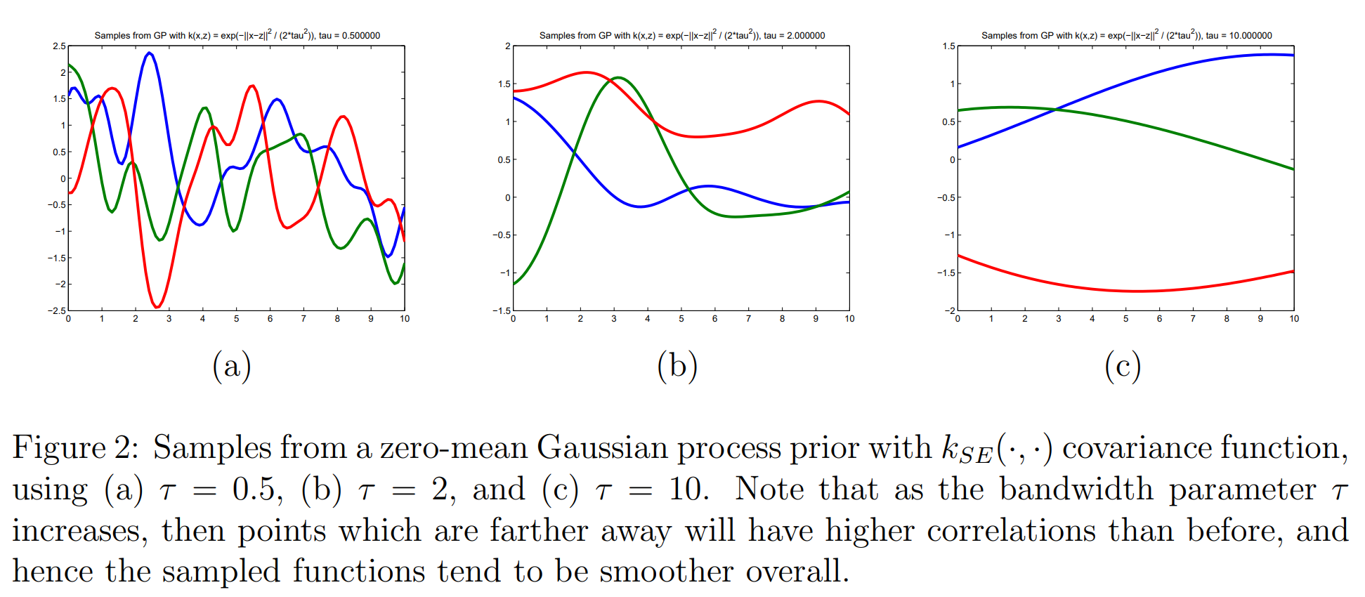
\[h(\cdot) \sim \mathcal{GP}(0, \; k(\cdot, \cdot))\]이때, function $h$는 $h: \mathbb{R} \rightarrow \mathbb{R}$의 함수이다. 그리고 kernel function $k(\cdot, \cdot)$은 <squared exponential kernel function>3을 사용한다.
\[k_{SE}(x, x') = \exp \left( - \frac{1}{2\tau^2} (x - x')^2 \right) \quad (\tau > 0)\]이때, 위와 같은 GP에서 sample한 function $h(x)$는 어떻게 생겼을까? 먼저 함수값의 평균이 0이기 때문에 함수값이 0 주변에 분포할 것이라고 생각할 수 있다. 또, $x, x’ \in \mathcal{X}$인 두 원소에 대한 함수값은
- $x$와 $x’$가 가깝다(nearby)면, $k_{SE}(x, x’) \approx 1$이 되므로 $h(x)$와 $h(x’)$는 high covariance를 가진다.
- 반대로 $x$와 $x’$가 멀다(far apart)면, $k_{SE}(x, x’) \approx 0$이 되므로 $h(x)$와 $h(x’)$는 low covariance를 가진다.
이런 아이디어를 바탕으로 실제로 샘플링 해보면 아래와 같다고 한다.
자! 여기까지 <Gaussian Process>에 대해 살펴보았다. distribution over random vector의 개념을 확장한 distribution over random function 그리고 그것을 infinite dimension까지 확장한 Gaussian Process까지!! 이번 포스트에서 다룬 내용이 결코 쉽지는 않지만, 공부할 가치는 충분한 주제였다 💪
다음 포스트에선 GP를 이용해 Regression model을 만드는 <Gaussian Process Regression>에 대해 살펴본다!!
references
-
이전의 <Bernoulli Process>의 경우, 각 trial에서 모두 동일한 <Bernoulli distribution>을 가정했는데, <Gaussian Process>의 경우 $x$ 값에 따라 다른 평균/분산을 가진 Gaussian distribution으로 이뤄질 수 있음에 주목하자! ↩
-
보통 <Gaussian Process>의 정확한 정의는 이 문장으로 표현한다. “A Gaussian process is a stochastic process s.t. any finite subcollection of random variables has a multivariate Gaussian distribution.” ↩
-
사실 SE kernel은 gaussian kernel의 한 종류이다. 다만, 여기서는 Gaussian Process와 이름이 겹쳐서 squared-exponential라는 이름을 쓰게 되었다. ↩