
Student’s t-distribution
“확률과 통계(MATH230)” 수업에서 배운 것과 공부한 것을 정리한 포스트입니다. 전체 포스트는 Probability and Statistics에서 확인하실 수 있습니다 🎲
시리즈: Sampling Distributions
Student’s t-distribution
Definition. Student’s t-distribution
Let $Z \sim N(0, 1)$, and $V \sim \chi^2(n)$, and $Z \perp V$.
Define $T$ as
\[T := \frac{Z}{\sqrt{V / n}}\]Then, the distribution of $T$ is called <student’s t-distribution of $n$ degrees of freedom>.
정의가 조금 복잡하긴 한데, 일단 서로 독립인 표준 정규 분포와 카이 제곱 분포의 조합으로 t-분포가 만들어진다~ 라는 감만 잡고 넘어갑시다.
t-분포 쪽은 이후에 나올 구간 추정에서 sample variance $s^2$를 사용할 줄 아는게 훨씬 더 중요합니다.
Remark.
1. The pdf of $t$-distribution is
\[f(x) = \frac{\Gamma\left(\dfrac{n+1}{2}\right)}{\sqrt{n\pi} \cdot \Gamma\left( \dfrac{n}{2} \right)} \left( 1 + \frac{x^2}{n} \right)^{-(n+1)/2}\]for $x \in \mathbb{R}$.
걱정하지 마라, 학부 수준에서 t-분포의 pdf를 외워서 사용할 일은 절대 없다!
2. $t$-distribution would converges to normal distribution as $n \rightarrow \infty$.
\[t(x; n) \rightarrow \frac{1}{\sqrt{2\pi}} \cdot \exp(-x^2 / 2)\]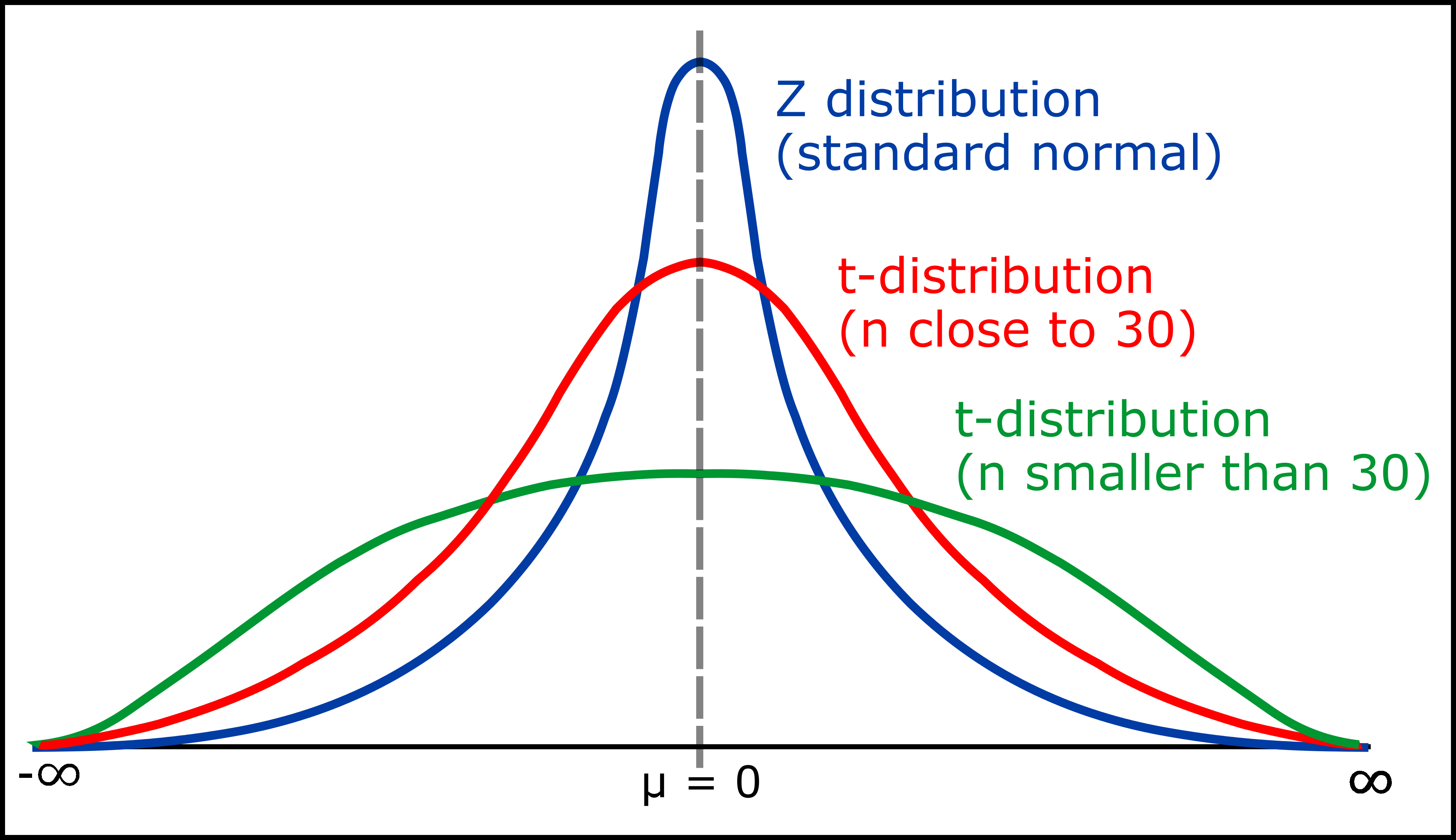
$n$이 커질 수록 정규 분포에 가까워진다!
proof.
항목 별로 극한을 생각해보자.
[Step 1]
더 쉬운 녀석인 오른쪽 녀석부터 하겠다.
\[\left( 1 + \frac{x^2}{n} \right)^{-(n+1)/2}\]$\exp(x)$ 함수의 정의를 이용하자.
\[\left( 1 + \frac{x^2}{n} \right)^{-n/2} \cdot \left( 1 + \frac{x^2}{n} \right)^{-1/2}\]$n \rightarrow \infty$일 때, 왼쪽은
\[\left( 1 + \frac{x^2}{n} \right)^{-n/2} \rightarrow \exp(-x^2 / 2)\]오른쪽은
\[\left( 1 + \frac{x^2}{n} \right)^{-1/2} \rightarrow (1)^{-1/2} = 1\]따라서,
\[\left( 1 + \frac{x^2}{n} \right)^{-(n+1)/2} \rightarrow \exp(-x^2 / 2)\][Step 2]
\[\frac{\Gamma\left(\dfrac{n+1}{2}\right)}{\sqrt{n\pi} \cdot \Gamma\left( \dfrac{n}{2} \right)}\]감마 함수는 아래와 같이 생겼다.
\[\Gamma(\alpha) = \int^{\infty}_0 t^{\alpha - 1} e^{-t} dt \quad \text{for} \; \alpha > 0\]여기서 그냥 받아들여야 하는 부분이 등장하는데, 바로 <스털링 근사; Stirling’s Approximation>다.
<스털링 근사>에 따르면, 큰 $k$에 대해 아래가 성립한다.
\[\Gamma(k) \approx \sqrt{\frac{2\pi}{k}} \left( \frac{k}{e} \right)^k\]이 사실을 바탕으로 수식을 전개하면,
\[\begin{aligned} \frac{\Gamma\left(\dfrac{k+1}{2}\right)}{\Gamma\left( \dfrac{k}{2} \right)} &= \frac{ \sqrt{\frac{1}{k + 1}} \left( \frac{k + 1}{2e} \right)^{(k+1) / 2} }{ \sqrt{\frac{1}{k}} \left( \frac{k}{2e} \right)^{k/2} } \\ &= \sqrt{\frac{k}{k+1}} \cdot \frac{(2e)^{k/2}}{(2e)^{(k+1)/2}} \cdot \frac{(k+1)^{(k+1)/2}}{(k)^{k/2}} \\ &= \sqrt{\frac{k}{k+1}} \cdot \frac{1}{\sqrt{2e}} \cdot \left(\frac{k+1}{k}\right)^{k/2} \cdot \sqrt{k+1} \\ &= \sqrt{\frac{k}{2e}} \cdot \left(1 + \frac{1}{k}\right)^{k/2} \\ \end{aligned}\]이제 수식을 합치면,
\[\begin{aligned} \frac{\Gamma\left(\dfrac{n+1}{2}\right)}{\sqrt{n\pi} \cdot \Gamma\left( \dfrac{n}{2} \right)} &= \frac{1}{\sqrt{n \pi}} \cdot \sqrt{\frac{n}{2e}} \cdot \left(1 + \frac{1}{n}\right)^{n/2} \\ &\rightarrow \frac{1}{\sqrt{\pi}} \cdot \sqrt{\frac{1}{2e}} \cdot \sqrt{e} \\ &= \frac{1}{\sqrt{2\pi}} \end{aligned}\][Final]
종합하면,
\[\begin{aligned} f(x) &= \frac{\Gamma\left(\dfrac{n+1}{2}\right)}{\sqrt{n\pi} \cdot \Gamma\left( \dfrac{n}{2} \right)} \cdot \left( 1 + \frac{x^2}{n} \right)^{-(n+1)/2} \\ &\rightarrow \frac{1}{\sqrt{2\pi}} \cdot \exp(-x^2 / 2) \end{aligned}\]3. We define $t_\alpha$ as the number $x$ s.t. $P(T \ge x) = \alpha$.
3번은 표기에 대한 걸로 이후에 t-분포를 사용해 구간 추정을 할 때, 이 기호를 사용합니다.
Sampling Distribution of Sample Mean (unknown $\sigma^2$)
Sample Mean $\bar{X}$에 대한 분포를 계속 살펴보자. 이전의 “Sampling Distribution of Sample Mean” 포스트에선 population variance $\sigma^2$에 대한 값을 정확히 알고 있었다.
\[Z = \frac{\bar{X} - \mu}{\sigma / \sqrt{n}} \sim N(0, 1)\]이번에는 $\sigma^2$를 모르는 상태에서 Sample Mean $\bar{X}$의 분포를 모델링 해보자.
Theorem.
Let $X_1, \dots, X_n$ be a random sample from $N(\mu, \sigma^2)$1.
Let $T := \dfrac{\bar{X} - \mu}{S / \sqrt{n}}$, then $T$ has a t-distribution with $(n-1)$ dof.
Proof.
이때, 분자인 $\dfrac{\overline{X} - \mu}{\sigma / \sqrt{n}}$는 $N(0, 1)$의 분포를 따르고,
분모인 $S / \sigma$는
\[\frac{S}{\sigma} = \sqrt{\frac{(n-1) \cdot S^2}{\sigma^2}\cdot \frac{1}{(n-1)}}\]인데 이때, $\dfrac{(n-1)\cdot S^2}{\sigma^2}$가 $\chi^2(n-1)$를 따르므로.
식을 정리하면 분포 $T$는 아래와 같은데,
\[T = \frac{Z}{\sqrt{V/(n-1)}}\]$Z \sim N(0, 1)$이고 $V \sim \chi^2(n-1)$이다. 그리고 Sample Variance와 Sample Mean이 서로 독립이므로, $Z \perp V$이다.
따라서, $T$는 dof가 $n-1$인 t-distribution이다. $\blacksquare$
Examples
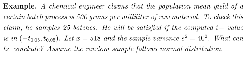
[population] $X$ follows Normal Distribution, $\mu = 500$, $\sigma$: unknown
[sample] $n=25$, $\bar{x} = 518$, $s^2 = 40^2$
[t-test] check weather or not $t \in [-t_{0.05}, t_{0.05}]$
Let $T := \dfrac{\bar{x} - \mu}{S / \sqrt{n}} \overset{D}{=} t(n-1) = t(24)$
t-value is
\[\frac{\bar{x} - \mu}{s/\sqrt{n}} = \frac{518-500}{40/5} = 2.25\]Here, $t_{0.05}(24) = 2.172$, and $t_{0.05} < 2.25$.
t-value가 $t_{0.05}$보다 크므로 유의하다. 그래서 population mean $\mu$는 500보다 더 클지도 모른다. $\blacksquare$
맺음말
이어지는 포스트에서는 두 sample variance를 비교할 때 쓰는 <F-distribution>를 살펴본다.
\[F := \frac{S_1^2 / \sigma_1^2}{S_2^2 / \sigma_2^2} = F(n_1 - 1, n_2 -1)\]<t-distribution>은 뒤에 나오는 <Interval Estimation>에서 다시 볼 예정이다.
👉 t-test: Estimate $\mu$ when $\sigma^2$ is unknown
개인적으로 여기가 <t-value>, <z-value>, <p-value>가 헷갈리는 지점이라고 생각한다. 만약, 두 개념이 어떻게 다르고, 또 언제 등장하는지 비교하고 싶다면, 아래의 포스트를 참고하길 바란다.
References
-
<t-distribution>을 쓰기 위해선, 샘플이 반드시 normal 분포로부터 추출되어야 한다!! 💥 ↩